Download

1 / 86
1.67k likes | 3.27k Views
Chapter 12 FLOW IN OPEN CHANNELS. A broad coverage of topics in open-channel flow has been selected for this chapter.

E N D
A broad coverage of topics in open-channel flow has been selected for this chapter. • In this chapter open-channel flow is first classified and then the shape of optimum canal cross sections is discussed, followed by a section on flow through a floodway. The hydraulic jump and its application to stilling basins is then treated, followed by a discussion of specific energy and critical depth which leads into transitions and then gradually varied flow. • Water-surface profiles are classified and related to channel control sections. In conclusion positive and negative surge waves in a rectangular channel are analyzed, neglecting effects of friction. • The presence of a free surface makes the mechanics of flow in open channels more complicated than closed-conduit flow. The hydraulic grade line coincides with the free surface, and, in general, its position is unknown.
For laminar flow to occur, the cross section must be extremely small, the velocity very small, or the kinematic viscosity extremely high. • One example of laminar flow is given by a thin film of liquid flowing down an inclined or vertical plane. Pipe flow has a lower critical Reynolds number of 2000, and this same value may be applied to an open channel when the diameter D is replaced by 4R, R is the hydraulic radius, defined as the cross-sectional flow area of the channel divided by the wetted perimeter. • In the range of Reynolds number, based on R in place of D, R = VR/v < 500 flow is laminar, 500 < R < 2000 flow is transitional and may be either laminar or turbulent, and R > 2000 flow is generally turbulent. • Most open-channel flows are turbulent, usually with water as the liquid. The methods for analyzing open-channel flow are not developed to the extent of those for closed conduits. The equations in use assume complete turbulence, with the head loss proportional to the square of the velocity.
12.1 CLASSIFICATION OF FLOW • Open-channel flow occurs in a large variety of forms, from flow of water over the surface of a plowed field during a hard rain to the flow at constant depth through a large prismatic channel. It may be classified as steady or unsteady, uniform or nonuniform. • Steady uniform flow occurs in very long inclined channels of constant cross section in those regions where terminal velocity has been reached, i.e., where the head loss due to turbulent flow is exactly supplied by the reduction in potential energy due to the uniform decrease in elevation of the bottom of the channel. • The depth for steady uniform flow is called the normal depth. In steady uniform flow the discharge is constant and the depth is everywhere constant along the length of the channel.
Steady nonuniform flow occurs in any irregular channel in which the discharge does not change with the time; it also occurs in regular channels when the flow depth and hence the average velocity change from one cross section to another. • For gradual changes in depth or section, called gradually varied flow, methods are available, by numerical integration or step-by-step means, for computing flow depths for known discharge, channel dimensions and roughness, and given conditions at one cross section. • Unsteady uniform flow rarely occurs in open-channel flow. Unsteady nonuniform flow is common but difficult to analyze. Wave motion is an example of this type of flow, and its analysis is complex when friction is taken into account.
Flow is also classified as tranquil or rapid. When flow occurs at low velocities so that a small disturbance can travel upstream and thus change upstream conditions, it is said to be tranquil flow (the Froude number F < 1). Conditions upstream are affected by downstream conditions, and the flow is controlled by the downstream conditions. • When flow occurs at such high velocities that a small disturbance, such as an elementary wave is swept downstream, the flow is described as shooting or rapid (F > 1). Small changes in downstream conditions do not effect any change in upstream conditions; hence, the flow is controlled by upstream conditions. • When flow is such that its velocity is just equal to the velocity of an elementary wave, the flow is said to be critical (F = 1). • The terms "subcritical" and "supercritical" are also used to classify flow velocities. Subcritical refers to tranquil flow at velocities less than critical, and supercritical corresponds to rapid flows when velocities are greater than critical.
Velocity Distribution • The velocity at a solid boundary must be zero, and in open-channel flow it generally increases with distance from the boundaries. • The maximum velocity does not occur at the free surface but is usually below the free surface a distance of 0.05 to 0.25 of the depth. • The average velocity along a vertical line is sometimes determined by measuring the velocity at 0.6 of the depth, but a more reliable method is to take the average of the velocities at 0.2 and 0.8 of the depth, according to measurements of the U.S. Geological Survey.
12.2 BEST HYDRAULUIC CHANNEL CROSS SECTIONS • Some channel cross sections are more efficient than others in that they provide more area for a given wetted perimeter. • From the Manning formula it is shown that when the area of cross section is a minimum, the wetted perimeter is also a minimum, and so both lining and excavation approach their minimum value for the same dimensions of channel. • The best hydraulic section is one that has the least wetted perimeter or its equivalent, the least area for the type of section. • The Manning formula is (12.2.1) • in which Q is the discharge (L3/T), A the cross-sectional flow area, R (area divided by wetted perimeter P) the hydraulic radius, S the slope of energy grade line, n the Manning roughness factor, Cm an empirical constant (L1/3/T) equal to 1.49 in USC units and to 1.0 in SI units.
With Q, n, and S known, Eq. (12.2.1) can be written (12.2.2) • in which c is known. This equation shows that P is a minimum when A is a minimum. • To find the best hydraulic section for a rectangular channel (Fig. 12.1) P = b + 2y and A = by. Then • Differentiating with respect to y gives • Setting dP/dy = 0 gives P = 4y, or since P = b + 2y, (12.2.3) • Therefore, the depth is one-half the bottom width, independent of the size of rectangular section.
To find the best hydraulic trapezoidal section (Fig. 12.2) A = by + my2, P = b + 2y√(1 + m2). After eliminating b and A in these Eq`ns and Eq. (12.2.2), (12.2.4) • By holding m constant and by differentiating with respect to y, ∂P/∂y is set equal to zero; thus (12.2.5) • Eq. (12.2.4) is differentiated with respect to m, and ∂P/∂m is set equal to zero, producing • And after substituting for m in Eq. (12.2.5), (12.2.6)
Figure 12.1 Rectangular cross section Figure 12.2 Trapezoidal cross section
Example 12.1 • Determine the dimensions of the most economical trapezoidal brick-lined channel to carry 200 m3/s with a slope of 0.0004. Solution • With Eq. (12.2.6), • and by substituting into Eq. (12.2.1) • or • and from Eq. (12.2.6) b = 7.5 m.
12.3 STEADY UNIFORM FLOW IN A FLOODWAY • A practical open-channel problem of importance is the computation of discharge through a floodway (Fig. 12.3). In general, the floodway is much rougher than the river channel and its depth (and hydraulic radius) is much less. The slope of energy grade line must be the same for both portions. • The discharge for each portion is determined separately, using the dashed line of Fig. 12.3 as the separation line for the two sections (but not as solid boundary), and then the discharges are added to determine the total capacity of the system. Figure 12.3 Floodway cross section
Since both portions have the same slope, the discharge may be expressed as or (12.3.1) • in which the value of K is • from Manning's formula and is a function of depth only for a given channel with fixed roughness. By computing K1 and K2 for different elevations of water surface, their sum may be taken and plotted against elevation. • From this plot it is easy to determine the slope of energy grade line for a given depth and discharge from Eq. (12.3.1).
12.4 HYDRAULIC JUMP; STILLING BASINS • The relations among the variables V1, y1, V2, y2 for a hydraulic jump to occur in a horizontal rectangular channel are developed before. Another way of determining the conjugate depths for a given discharge is the F + M method. • The momentum equation applied to the free body of liquid between y1 and y2 (Fig. 12.4) is, for unit width (V1y1 = V2y2 = q), • Rearranging gives (12.4.1) • or (12.4.2) • F is the hydrostatic force at the section and M is the momentum per second passing the section.
By writing F + M for a given discharge q per unit width (12.4.3) • a plot is made of F + M as abscissa against y as ordinate (Fig. 12.5) for q = 1 m3/s · m. Any vertical line intersecting the curve cuts it at two points having the same value of F + M; hence, they are conjugate depths. • The value of y for minimum F + M is (12.4.4) • This depth is the critical depth, which is shown in the following section to be the depth of minimum energy. Therefore, the jump always occurs from rapid flow to tranquil flow.
Figure 12.4 Hydraulic jump in horizontal rectangular channel Figure 12.5 F + M curve for hydraulic jump
The conjugate depth are directly related to the Froude number before and after the jump, (12.4.5) • From the continuity equation • or (12.4.6) • From Eq. (12.4.1) • Substituting from Eqs. (12.4.5) and (12.4.6) gives (12.4.7)
The value of F2 in terms of F1 is obtained from the hydraulic-jump equation • By Eqs. (12.4.5) and (12.4.6) (12.4.8) • These equations apply only to a rectangular section. • The Froude number is always greater than unity before the jump and less than unity after the jump.
Stilling Basins • A stilling basin is a structure for dissipating available energy of flow below a spillway, outlet works, chute, or canal structure. In the majority of existing installations a hydraulic jump is housed within the stilling basin and used as the energy dissipator. • This discussion is limited to rectangular basins with horizontal floors although sloping floors are used in some cases to save excavation. See table 12.1 • Baffle blocks are frequently used at the entrance to a basin to corrugate the flow. They are usually regularly spaced with gaps about equal to block widths. • Sills, either triangular or dentated, are frequently employed at the downstream end of a basin to aid in holding the jump within the basin and to permit some shortening of the basin. • The basin should be paved with high-quality concrete to prevent erosion and cavitation damage. No irregularities in floor or training walls should be permitted.
Table 12.1 Classification of the hydraulic jump as an effective energy dissipator
Example 12.2 • A hydraulic jump occurs downstream from a 15-m-wide sluice gate. The depth is 1.5 m, and the velocity is 20 m/s. Determine (a) the Froude number and the Froude number corresponding to the conjugate depth, (b) the depth and velocity after the jump, and (c) the power dissipated by the jump. Solution (a) • From Eq. (12.4.8) (b)
Then • and (c) • Form Eq. (3.11.24), the head loss hj in the jump is • The power dissipated is
12.5 SPECIFIC ENERGY; CRITICAL DEPTH • The energy per unit weight Es with elevation datum taken as the bottom of the channel is called the specific energy. It is plotted vertically above the channel floor, (12.5.1) • A plot of specific energy for a particular case is shown in Fig. 12.6. In a rectangular channel, in which q is the discharge per unit width, with Vy = q, (12.5.2) • It is of interest to note how the specific energy varies with the depth for a constant discharge (Fig. 12.7). • For small values of y the curve goes to infinity along the Es axis, while for large values of y the velocity head term is negligible and the curve approaches the 450 line Es = y asymptotically.
Figure 12.6 Example of specific energy Figure 12.7 Specific energy required for flow of a given discharge at various depths.
The value of y for minimum Es is obtained by setting dEs /dy equal to zero, from Eq. (12.5.2), holding q constant, • or (12.5.3) • The depth for minimum energy yc is called critical depth. Eliminating q2 in Eqs. (12.5.2) and (12.5.3) gives (12.5.4) • showing that the critical depth is two-thirds or the specific energy. Eliminating Es in Eqs. (12.5.1) and (12.5.4) gives (12.5.5) • Another method of arriving at the critical condition is to determine the maximum discharge q that could occur for a given specific energy. The resulting equations are the same as Eqs. (12.5.3) to (12.5.5).
For nonrectangular cross sections, as illustrated in Fig. 12.8, the specific-energy equation takes the form (12.5.6) • in which A is the cross-sectional area. To find the critical depth • From Fig. 12.8, the relation between dA and dy is expressed by • in which T is the width of the cross section at the liquid surface. With this relation (12.5.7)
The critical depth must satisfy this equation. Eliminating Q in Eqs. (12.5.6) and (12.5.7) gives (12.5.8) • This equation shows that the minimum energy occurs when the velocity head is one-half the average depth A/T. Equation (12.5.7) may be solved by trail for irregular sections by plotting • Critical depth occurs for that value of y which makes f(y) = 1.
Example 12.3 • Determine the critical depth for 10 m3/s flowing in a trapezoidal channel with bottom width 3 m and side slopes 1 horizontal to 2 vertical (1 on 2). Solution • Hence • By trail • The critical depth is 0.984 m. This trail solution is easily carried out by programmable calculator.
12.6 TRANSITIONS • At entrances to channels and at changes in cross section and bottom slope, the structure that conducts the liquid from the upstream section to the new section is a transition. • Its purpose is to change the shape of flow and surface profile in such a manner that minimum losses result. • A transition for tranquil flow from a rectangular channel to a trapezoidal channel is illustrated in Fig. 12.10. Applying the energy equation from section 1 to section 2 gives (12.6.1) • In general, the sections and depths are determined by other considerations, and z must be determined for the expected available energy loss E1 .
Figure 12.10 Transition from rectangular channel to trapezoidal channel for tranquil flow
Example 12.5 • In Fig. 12.10, 11 m3/s flows through the transition; the rectangular section 2.4 m wide; and y1 = 2.4 m. The trapezoidal section is 1.8 m wide at the bottom with side slopes 1 : 1, and y2 = 2.25 m. Determine the rise z in the bottom through the transition. • Solution • Substituting into Eq. (12.6.1) gives
The critical-depth meter is an excellent device for measuring discharge in an open channel. The relations for determination of discharge are worked out for a rectangular channel of constant width, Fig. 12.11, with a raised floor over a reach of channel about 3yc long. • Applying the energy equation from section 1 to the critical section (exact location unimportant), including the transition-loss term, gives • Since • In which Ec is the specific energy at critical depth, (12.6.2)
From Eq. (12.5.3) (12.6.3) • In Eqs. (12.6.2) and (12.6.3) Ec is eliminated and the resulting equation solved for q, • Since q = V1y1, V1 can be eliminated, (12.6.4) • The equation is solved by trial. As y1 and z are known and the right-hand term containing q is small, it may first be neglected for an approximate q. A value a little larger than the approximate q may be substituted on the right-hand side. When the two q 's are the same the equation is solved. • Experiments indicate that accuracy within 2 to 3 percent may be expected.
Example 12.6 • In a critical-depth meter 2 m wide with z = 0.3 m the depth y1 is measured to be 0.75 m. Find the discharge. Solution • As a second approximation let q be 0.50, • And as a third approximation, 0.513, • Then
12.7 GRADUALLY VARIED FLOW • Gradually varied flow is steady nonuniform flow of a special class. The depth, area, roughness, bottom slope, and hydraulic radius change very slowly (if at all) along the channel. • Solving Eq. (12.2.1) for the head loss per unit length of channel produces (12.7.1) • in which S is now the slope of the energy grade line or, more specifically, the sine of the angle the energy grade line makes with the horizontal. • Computations of gradually varied flow may be carried out either by the standard-step method or by numerical integration. Horizontal channels of great width are treated as a special case that may be integrated.
Standard-Step Method • Applying the energy equation between two sections a finite distance ΔL apart (Fig. 12.12), including the loss term, gives (12.7.2) • Solving for the length of reach gives (12.7.3) • If conditions are known at one section, e.g., section 1, and the depth y2 is wanted a distance ΔL away, a trial solution is required. The procedure is as follows: • Assume a depth y2; then compute A2, V2. • For the assumed y2 find an average y, P, and A for the reach and compute S. • Substitute in Eq. (12.7.3) to compute ΔL. • If ΔL is not correct, assume a new y2 and repeat the procedure.
The standard-step method is easily followed with the programmable calculator if about 20 memory storage spaces and about 100 program steps are available. • In the first trial y2 is used to evaluate ΔLnew. Then a linear proportion yields a new trial y2new for the next step; thus or • A few iterations yield complete information on section 2.
Example 12.7 • At section 1 of a canal the cross section is trapezoidal, b1 = 10 m, m1 = 2, y1 = 7 m, and at section 2, downstream 200 m, the bottom is 0.08 m higher than at section 1, b2 = 15 m, and m2 = 3. Q = 200 m3/s, n = 0.035. Determine the depth of water at section 2. Solution • Since the bottom has an adverse slope, i.e.. it is rising in the downstream direction, and since section 2 is larger than section 1, y2 is probably less than y1. Assume y2 = 6.9 m; then • and
The average A = 207 and average wetted perimeter P = 50.0 are used to find an average hydraulic radius for the reach, R = 4.14 m. Then • Substituting into Eq. (12.7.3) gives • A larger y2, for example, 6.92 m, would bring the computed value of length closer to the actual length.
Numerical Integration Method • A more satisfactory procedure, particularly for flow through channels having a constant shape of cross section and constant bottom slope, is to obtain a differential equation in terms of y and L and then perform the integration numerically. • When ΔL is considered as an infinitesimal in Fig. 12.12, the rate of change of available energy equals rate of head loss -ΔE/ΔL given by Eq. (12.7.1), or (12.7.4) • in which z0 – S0L is the elevation of bottom of channel at L, z0 is the elevation of bottom at L = 0, and L is measured positive in the downstream direction. • After performing the differentiation, (12.7.5)
Using the continuity equation VA = Q leads to • And expression dA = T dy, in which T is the liquid–surface width of the cross section, gives • Substituting for V in Eq. (12.7.5) yields • And solving for dL gives (12.7.6)
After integrating, (12.7.7) • In which L is the distance between the two sections having depths y1and y2. • When the numerator of the integrand is zero, critical flow prevails; there is no change in L for a change in y (neglecting curvature of the flow and nonhydrostatic pressure distribution at this section ). Since this is not a case of gradual change in depth, the equations are not accurate near critical depth. • When the denominator of the integrand is zero, uniform flow prevails and there is no change in depth along the channel. The flow is at normal depth.
For a channel of prismatic cross section, constant n and S0, the integrand becomes a function of y only, • and the equation can be integrated numerically by plotting F(y) as ordinate against y as abscissa. • The area under the curve (Fig. 12.13) between two values of y is the length L between the sections, since
Figure 12.13 Numerical integration of equation for gradually varied flow
Example 12.8 • A trapezoidal channel, b = 3 m, m = 1, n = 0.014, S0 = 0.001, carries 28 m3/s. If the depth is 3 m at section 1, determine the water-surface profile for the next 700 m downstream. Solution • To determine whether the depth increases or decreases, the slope of the energy grade line at section 1 is computed using Eq. (12.7.1) • and • Then
Substituting into Eq. (12.5.7) the values A, Q and T = 9 m gives Q2T/gA3 = 0.12, showing that the depth is above critical. With the depth greater than critical and the energy grade line less steep than the bottom of the channel, the specific energy is increasing. • When the specific energy increases above critical, the depth of flow increases. Δy is then positive. Substituting into Eq. (12.7.6) yields • The following table evaluates the terms of the integrand.