Ocean Dynamics Algorithm GOES-R AWG

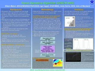
1. Ocean Dynamics Algorithm GOES-R AWG Eileen Maturi, NOAA/NESDIS/STAR/SOCD, Igor Appel, STAR/IMSG, Andy Harris, CICS, Univ of Maryland • Background • At present, there is no NOAA real-time single-sensor (imager) algorithm for ocean currents • However, feature tracking is performed to derive Atmospheric Motion Vectors on an operational basis • Difference for ocean currents is that speeds are 1-2 orders of magnitude slower than for winds • Thus image-to-image registration becomes critical • Note: All AWG algorithms are developed under the assumption of accurate calibration and navigation • Substantial “from scratch” development effort required for this Day 2 product • GOES-R ABI – key aspects • Imaging every 15 minutes (full-disk) • 16 bands, including several in thermal IR “window” • Spatial resolution of 2 km (for thermal IR) • Image navigation accuracy specification 750 m • Meteosat-8/9 SEVIRI – selected proxy • Chosen as best proxy data upon which to develop and test algorithm for this task: • “Similar” thermal bands • Resolution 3 km (for thermal IR) • 15-minute full-disk imaging • Spin-scan stabilization (vs. 3-axis for GOES-R Platform) – not clear what the actual image-to-image navigation accuracy is, but is thought to be “good” • Obviously not easy to test for regions of interest specific to US coastal waters • N.B. requirement is for 2 products: “Ocean Currents” and “Ocean Currents: Offshore” – the latter has US Exclusive Economic Zone masked • Methodology • Required accuracy is 0.3 m.s-1 for ocean current U & V components, 3-hour refresh rate The GOES-R ocean surface vector approach consists of the following general steps: • Locate and select a suitable target in second image (middle image; time=t0) of image triplet • Use a pattern matching algorithm to locate the target in an earlier and later image. Track target backward in time (to first image; time=t-Δt) and forward in time (to third image; time=t+Δt) and compute corresponding displacement vectors. Compute mean vector displacement valid at time = t0 • Perform quality assurance on ocean surface vectors. Flag suspect vectors. Compute and append quality indicators to each vector • Apply mask to get Offshore Currents • Validation • SEVIRI data centered at 12 UTC were selected for 8 days in each season (total 32 days) • A variety of target sizes were evaluated • Compare with currents from the global version of the Navy Coastal Ocean Model (NCOM) • Advantage of using model field is that vectors are available “everywhere” • Potential for model-related biases (e.g. displaced currents, errors in forcing fields). However, NCOM does assimilate data (e.g. Altimetry) and is therefore constrained by it • “Global” NCOM is high resolution (at least eddy-resolving) Example Ocean Current Vectors derived from MSG-SEVIRI image triplet centered at 12Z Vector length indicates derived current strength (1 degree = 1 m.s-1) Shows upwelling off N Africa, combined with complex current pattern in the vicinity of the Canary Islands July 8, 2005 North Africa Read GOES-R IR & SST data Orange = gaussian curve represented by S.D. Green = gaussian represented by R.S.D. Blue = histogram of errors (MSG – NCOM) 5×5 Target Median = 0.13 R.S.D. = 0.348 Median = 0.06 R.S.D. = 0.297 Apply Cloud Mask & Land Mask Ocean Currents Algorithm (feature detection, pattern matching – SSD*, vector derivation, QC) *SSD = Sum of Squared Differences Note: green curve matches peak & central distribution Inclusion of “weak” gradient targets degrades accuracy One solution to achieve 100% requirement is to QC output using gradient strength =0.5 =0.3 80% Output Ocean Current Vectors 100% Sum-of-Squared Differences (SSD) I1 = Temperature at pixel (x1,y1) of the target scene I2 = Temperature at pixel (x2,y2) of the search scene • Validation against HYCOM assimilation runs • Investigate: 1) impact of geolocation errors in proxy data; 2) alternative cloud mask; 3) alternative pattern matching & data assimilation approaches (OSU/CIOSS) Search Region Matching Scene • Summation is carried out for all possible target scene positions within the search region • The matching scene corresponds to the scene where the function takes on the smallest value Original Target Scene AMS 92ndAnnual Meeting, New Orleans, Louisiana,January 22-27, 2012