Download
1 / 50
580 likes | 920 Views
Chapter 3 Application of Derivatives. 3.1 Extreme Values of Functions. Absolute maxima or minima are also referred to as global maxima or minima. Examples. Extreme Value Theorem. The requirements in Theorems 1 that the interval be closed and finite, and

E N D
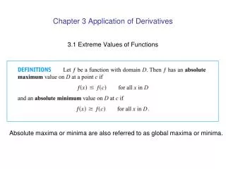
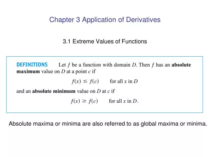
Chapter 3 Application of Derivatives 3.1 Extreme Values of Functions Absolute maxima or minima are also referred to as global maxima or minima.
Extreme Value Theorem The requirements in Theorems 1 that the interval be closed and finite, and That the function be continuous, are key ingredients.
Critical Point Theorem 2 says that a function’s first derivative is always zero at an interior point where the function has a local extreme value and the derivative is defined. Hence the only places where a function f can possibly have an extreme value (local or global) are • Interior points where f’=0 • Interior points where f’ is undefined, • Endpoints of the domain of f.
How to Find the Absolute Extrema Thus the only domain points where a function can assume extreme values are critical points and endpoints.
Example Example. Find the absolute maximum and minimum values of f(x)=10x(2-lnx) on the interval [1, ex]. Solution. We evaluate the function at the critical points and the endpoints and take the largest and the smallest of the resulting values. The first derivative is f’(x)=10(2-lnx)-10x(1/x)=10(1-lnx). Let f’(x)=0, we have x=e. Then Critical point value: f(e)=10e Endpoint values: f(1)=20, and f(e2)=0. So the function’s absolute maximum value is10e at x=e. The absolute minimum value is 0 and occurs at the right endpoint x=e2.
3.3 Monotonic Functions and the First Derivative Test A function that is increasing or decreasing on an interval is said to be monotonic on the interval.
Graphs of functions Each tangent line Has positive slope. Each tangent line Has negative slope. Each tangent line Has zero slope.
Example Example: Find the critical points of f(x)=x3 -12x-5 and identify the intervals on which f is increasing and on which f is decreasing.
Example Find the critical points of f(x)=(x2-3)ex. Identify the intervals on which f is increasing and decreasing. Find the function’s local and absolute extreme values. Solution.
3.4 Concavity and Curve Sketching • Two ways to characterize the concavity of a differentiable function f on an open interval: • f is concave up on an open interval if its tangent lines have increasing slopes on that interval and is concave down if they have decreasing slopes. • f is concave up on an open interval if its graph lies above its tangent lines on that interval and is concave down if it lies below its tangent lines
Concavity and the Second Derivative Test for Concavity If y=f(x) is twice-differentiable, we will use f’’ and y’’ interchangeable When denoting the second derivative.
Example Example: Find the intervals on which is concave up and the intervals on which it is concave down. Solution:
Second Derivative Test for Local Extrema This test requires us to know f’’ only at c itself and not in an interval about c. This makes the test easy to apply. However, this test is inconclusive if f’’=0 or if ‘’ does not exist at x=c. When this happens, use the First derivative Test for local extreme values.
Parametric Formula for dy/dx Example. Find dy/dx as a function of t if x = t - t2, y = t - t3. Solution.
3.6 Applied Optimization To optimize something often means to maximize or minimize some aspect of it. Example 1 An open-tup box is to be made by cutting small congruent squares from the corners of a 12-in.–by-12-in. sheet of tin and bending up the sides. How large should the squares cut from the corners be to make the box hold as much as possible?
Example 2: You have been asked to design a 1-liter can shaped like a right Circular cylinder. What dimensions will used the least material?
Example Example: Find
Example Example: Find
Example Example: Find
Example Example: Find
Sometimes when we try to evaluate a limit as xa by substituting x=a we get an ambiguous expression like . Sometimes these forms can be handled by using algebra to convert them to a o/o or form. For example: Find • (b)
Indeterminate Powers Limits that lead to the indeterminate forms can sometims be Handled by first taking the logarithm of the function. We use l’Hopital’s Rule to find the limit of the logarithm expression and then exponentiate the result to find the original function limit. Example: Find .
3.8 Newton’s Method (Optional) Newton’s method is a technique to approximate the solution to an equation f(x)=0. Essentially it uses tangent lines in place of the graph of y=f(x) near the points where f is zero. (A value of x where f is zero is a root of the function f and a solution of the equation f(x)=0.)
To find a root r of the equation f(x)=0, • select an initial approximation x1. If f(x1)=0, then r=x1. Otherwise, use the root of the tangent line to the graph of f at x1 to approximate r. Call this intercept x2 . • We can now treat x2 in the same way we did x1. If f(x2 )=0, then r= x2 . Otherwise, we construct the tangent line to the graph of f at x2, and take x3 to be the x-intercept of the tangent line. Continuing in this way, we can generate a succession of values x1,x2,,x3,,,x4…that will usually approach r.
Example Use Newton’s Method to approximate the real solutions of x3-x-1=0 Solution: