Download
1 / 46
500 likes | 664 Views
Chapter 3 Application of Derivatives. 3.1 Extreme Values of Functions. Absolute maxima or minima are also referred to as global maxima or minima. Examples. Extreme Value Theorem. The requirements in Theorems 1 that the interval be closed and finite, and

E N D
Chapter 3 Application of Derivatives 3.1 Extreme Values of Functions Absolute maxima or minima are also referred to as global maxima or minima.
Extreme Value Theorem The requirements in Theorems 1 that the interval be closed and finite, and That the function be continuous, are key ingredients.
Critical Point Theorem 2 says that a function’s first derivative is always zero at an interior point where the function has a local extreme value and the derivative is defined. Hence the only places where a function f can possibly have an extreme value (local or global) are • Interior points where f’=0 • Interior points where f’ is undefined, • Endpoints of the domain of f.
How to Find the Absolute Extrema Thus the only domain points where a function can assume extreme values are critical points and endpoints.
Example Example. Find the absolute maximum and minimum values of f(x)=10x(2-lnx) on the interval [1, ex]. Solution. We evaluate the function at the critical points and the endpoints and take the largest and the smallest of the resulting values. The first derivative is f’(x)=10(2-lnx)-10x(1/x)=10(1-lnx). Let f’(x)=0, we have x=e. Then Critical point value: f(e)=10e Endpoint values: f(1)=20, and f(e2)=0. So the function’s absolute maximum value is10e at x=e. The absolute minimum value is 0 and occurs at the right endpoint x=e2.
3.3 Monotonic Functions and the First Derivative Test A function that is increasing or decreasing on an interval is said to be monotonic on the interval.
Graphs of functions Each tangent line Has positive slope. Each tangent line Has negative slope. Each tangent line Has zero slope.
Example Example: Find the critical points of f(x)=x3 -12x-5 and identify the intervals on which f is increasing and on which f is decreasing. Solution: The function f is everywhere continuous and differentiable. The first derivative f ’(x)=3x2-12=3(x2-4)=3(x+2)(x-2) is zero at x=-2 and x=2. These critical points subdivide the domain of f into intervals (-, -2), (-2, 2) and (2, ) on which f ‘ is either positive or negative. We determine the sign Of f ‘ by evaluating f at a convenient point in each subinterval. Interval -<x<-2 -2<x<2 2<x< f ‘ evaluated f ’(-3) = 15 f ‘(0)=12 f ‘ (3) =15 Sign of f ‘ + - + Behavior of f increasing decreasing increasing
Example Find the critical points of f(x)=(x2-3)ex. Identify the intervals on which f is increasing and decreasing. Find the function’s local and absolute extreme values. Solution. f ’(x)=(x2+2x-3)ex. Since ex is never zero, f ‘(x) is zero iff x2+2x-3=0. That is, x=-3 and x=1. We can see that there is a local maximum about 0.299 at x=-3 and a local minimum about -5.437 at x=1. The local minimum value is also an absolute minimum, but there is no absolute maximum. The function increases on (-, -3) and (1, ) and deceases on (-3, 1).
3.4 Concavity and Curve Sketching • Two ways to characterize the concavity of a differentiable function f on an open interval: • f is concave up on an open interval if its tangent lines have increasing slopes on that interval and is concave down if they have decreasing slopes. • f is concave up on an open interval if its graph lies above its tangent lines on that interval and is concave down if it lies below its tangent lines
Concavity and the Second Derivative Test for Concavity If y=f(x) is twice-differentiable, we will use f’’ and y’’ interchangeable When denoting the second derivative.
Example Example: Find the intervals on which is concave up and the intervals on which it is concave down. Solution: Thus f(x) is concave up on the interval , and concave down on the interval
Second Derivative Test for Local Extrema This test requires us to know f’’ only at c itself and not in an interval about c. This makes the test easy to apply. However, this test is inconclusive if f’’=0 or if ‘’ does not exist at x=c. When this happens, use the First derivative Test for local extreme values.
Parametric Formula for dy/dx Example. Find dy/dx as a function of t if x = t - t2, y = t - t3. Solution.
Example Example: Find Solution: The limit is a indeterminate form of type 0/0. Applying L’Hopital’s rule yields
Example Example: Find Solution: The limit is a indeterminate form of type 0/0. Applying L’Hopital’s rule yields
Example Example: Find Solution: The limit is a indeterminate form of type Applying L’Hopital’s rule yields In fact, we can use LHopital’s rule to show that
Example Example: Find Solution: The limit is a indeterminate form of type Applying L’Hopital’s rule yields Similar methods can be used to find the limit of f(x)/g(x) is an Indeterminate form of the types:
3.8 Newton’s Method Newton’s method is a technique to approximate the solution to an equation f(x)=0. Essentially it uses tangent lines in place of the graph of y=f(x) near the points where f is zero. (A value of x where f is zero is a root of the function f and a solution of the equation f(x)=0.)
To find a root r of the equation f(x)=0, • select an initial approximation x1. If f(x1)=0, then r=x1. Otherwise, use the root of the tangent line to the graph of f at x1 to approximate r. Call this intercept x2 . • We can now treat x2 in the same way we did x1. If f(x2 )=0, then r= x2 . Otherwise, we construct the tangent line to the graph of f at x2, and take x3 to be the x-intercept of the tangent line. Continuing in this way, we can generate a succession of values x1,x2,,x3,,,x4…that will usually approach r.
Example Use Newton’s Method to approximate the real solutions of x3-x-1=0 Solution: Let f(x)=x3-x-1. Since f(1)=-1 and f(2)=5, weh know by the Intermediate Value Theorem, there is a root in the interval (1, 2). We apply Newton’s method to f with the starting values x0 =1. The result are displayed in the following table and figure.
At n=5, we come to the result x6=x5=1.324717957. When xn+1=xn, Equation (1) shows that f(xn)=0. We have found a folution of f(x)=0 to nine decimals.