Download
1 / 19
190 likes | 220 Views
This article discusses the implementation of the ADT Table and Heap data structures, their advantages and disadvantages, and how they can be used for various operations. It also explains the process of inserting and deleting items from a heap and provides an example of heap sort.

E N D
ADT Table and Heap Ellen Walker CPSC 201 Data Structures Hiram College
ADT Table • Represents a table of searchable items with at least one key (index) • E.g. dictionary, thesaurus, phone book • Value-based operations • Insert • Delete • Retrieve • Structural operations • Traverse (no specified order) • Create, destroy
Implementing a Table • Linear data structures • Unsorted array • Sorted array • Unsorted linked list • Sorted linked list • Tree • Binary search tree • Other • Hash table (ch. 12)
Issues to consider • Different structures are better for different operations • Sorted arrays and trees can be searched fastest • Linked lists and trees are easier to insert and delete • Sorted structures take longer for insertion than non-sorted structures • Consider simplicity of implementation, especially if the table is “small”
Restrictions Constrain Implementations • If we limit traversal to traversal in sorted order, we cannot use unsorted arrays or linked lists. • General rule: define the least restrictive set of operations that will satisfy needs; then choose an appropriate data structure • Example: heap vs. tree for priority queue
Priority Queue • Every item has a (numeric) priority • Multiple items can have the same priority • When dequeuing, the oldest item with the highest priority should be retrieved first • If all items of equal priority, then it is a queue • If all items different priority, it acts somewhat like a sorted list
Sorted Structure for Priority Queue • Items are kept sorted in reverse order (largest first) • To enqueue: insert item in place according to priority • To dequeue: remove first (highest) item • First item in reverse-sorted list or array • Last item in sorted list or array • Rightmost item in binary search tree
Heap: A new structure • A heap is a full binary tree • The root of the heap is larger than any node in either the left or right subtree • The left and right subtrees are both themselves heaps • An empty tree is a heap (base case)
Heap is less restrictive • Given a set of values, there are more possible heaps than there are binary search trees for the same set of values (why?) • When inserting an item into a heap, we don’t have to find its exact location in the sort order • We do have to make sure the heap property holds for the tree and all its subtrees • We only have to worry about deleting the root
Heap in Array • Because a heap is a full binary tree, it represents very well in an array • Root is heap[0] • Children of heap[k] are • heap[2*k+1] • heap[2*k+2] • Values are packed into the array (no holes)
An example heap • 21 17 5 12 9 4 3 11 10 2 21 17 5 12 4 3 9 11 10 2
Deleting • Remove the root (now you have a semiheap) • Replace the root by the last (bottom, rightmost) element • Swap root with largest child recursively until root is largest. • New root item “trickles down” a path until it finds its correct (sorted in the path) location
Example Deletion 2 17 17 5 12 5 12 4 3 9 11 4 3 9 11 10 2 10 Root replaced Heap property restored
Inserting into a Heap • Put new item at first available position at deepest level (last element in the array) • If it is larger than its parent, swap them • Continue swapping up the tree until the parent is larger or the new item has become the root.
Example Insertion 17 17 12 14 5 5 11 12 4 3 11 4 3 9 14 2 9 2 10 10 New item (14) at bottom Heap property restored
Efficiency of Heap • Adding • Element starts at the bottom, takes a single path from the bottom to the root (at most) • This is O(log N) because the tree is balanced (every path is <= log N + 1) • Removing • Element starts at the root, takes a single path down the tree • Again, O(log N)
Heap Sort • Begin with an array (in arbitrary order) • Make the array into a valid heap • Starting at the next-to-bottom level, rearrange “triples” so the local root is largest • Essentially, this works backwards in the array • While(heap is not empty) • Delete the root (and swap it with the last leaf) • Since the root is largest (each time), in the end, the array will be sorted
Example • Initial Array: • X W Z A R C D M Q E F • Initial heap: X W Z A R C D M Q E F
MaxHeap & MinHeap • We’ve been looking at MaxHeap • Largest item at root • Highest number is highest priority • Textbook describes MinHeap • Smallest item at root • Lowest number is highest priority • The only difference in algorithm is “max” vs. “min”