Quantized State System Simulation in Dymola/Modelica Using the DEVS Formalism

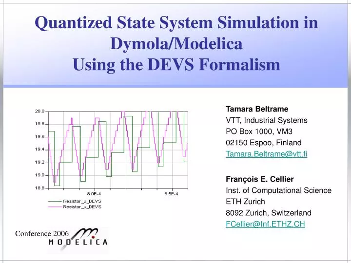
1. Tamara Beltrame VTT, Industrial Systems PO Box 1000, VM3 02150 Espoo, Finland Tamara.Beltrame@vtt.fi Conference 2006 Quantized State System Simulation in Dymola/ModelicaUsing the DEVS Formalism François E. Cellier Inst. of Computational Science ETH Zurich 8092 Zurich, Switzerland FCellier@Inf.ETHZ.CH

2. Abstract • A tool has been created for the simulation of highly discontinuous models in Dymola/Modelica that is based on Zeigler’s DEVS (Discrete Event Systems) formalism. • ModelicaDEVS provides a reimplementation of the PowerDEVS software, a tool developed for the simulation of physical systems that is based on Kofman’s QSS (Quantized State Systems) algorithms.

3. Overview • Motivation • The DEVS Formalism • Quantized State Systems • ModelicaDEVS • Simulation Results • Conclusions

4. Motivation • When simulating continuous models on a digital computer, a quantization must take place, as digital computers can only perform a finite number of computations within any finite time span. • Usually, it is the time axis that is being discretized, i.e., we are asking ourselves: given the current state at timet*, what value shall the state vector assume at timet* + h? • Yet, it is also possible to discretize the state axes, i.e., we can ask the question: given the current value of the quantized state variableqi, what is the earliest time when the variable will assume a value ofqi± Δqi?

5. Motivation 2 • Numerical simulation algorithms can be based on either paradigm. • Whereas almost all simulation algorithms currently on the market are based on the former approach, the QSS techniques are based on the latter. • The QSS approach has some distinct advantages: • The method is naturally asynchronous. • QSS simulations can be more easily combined with discrete events. • Most state events turn into time events in QSS. • A QSS simulation of an analytically stable system is always stable. • QSS offers a global error bound. • It is possible to design “implicit” algorithms that are not truly implicit.

6. The DEVS Formalism • DEVS was introduced by B. Zeigler in 1976. • DEVS is one among several discrete-event simulation methodologies. Other discrete-event techniques include: Petri nets, finite state machines, Markov chains, ... • Specialty: DEVS models work with an infinite number of states. This is useful for numerical integration.

7. The DEVS Formalism 2 Atomic Models • Accept an input trajectory (external event), generate an output trajectory. • Definition: M = <X, Y, S, δint, δext, λ, ta> • X = set of inputs • S = set of possible states • Y = set of outputs • δext = external transition • ta = time-advance function, often represented by σ • δint = internal transition • λ = output function

8. The DEVS Formalism 3 Atomic Models (cont.) Example:

9. The DEVS Formalism 4 Coupled Models • DEVS is closed under coupling. • Useful to split a complex model into simpler models. • The dynamics of the coupled model N: • Evaluate the atomic model d* that is the next one to execute an internal transition. Let tn be the time when the transition has to take place. • Advance the simulation time to t = tn and let d* execute the internal transition. • Forward the output of d* to all connected atomic models and let them execute their external transitions.

10. The DEVS Formalism 5 Hierarchical Models • Reuse of coupled models as atomic models. • The actual task of N is to wrap Ma and Mb, in order to make them look like they were one single model. • The coupled model N features the same transitions as an atomic model, but the transitions of N depend on the transitions of its sub-models.

11. Quantized State Systems (QSS) • QSS operate on piecewise constant input and output trajectories. • Systems with piecewise constant trajectories can be simulated using the DEVS formalism. • QSS use a quantization function to transform a continuous system into a system with piecewise constant input and output trajectories. • The quantization function is hysteretic in order to avoid illegitimate models. • Illegitimate models perform an infinite number of transitions in a finite time interval.

12. Quantized State Systems 2 Hysteretic Quantization Function • A quantization function maps real numbers x(t) into a discrete set of real values q(t). • Problem: x(t) = −sign(q(t)) • A hysteretic quantization function prevents infinite oscillations from occurring within a single time step. .

13. Quantized State Systems 3 Discretization of a Continuous System • Conventional continuous system: x(t) = f(x(t), u(t), t) • Quantized continuous system: ξ(t) = f(q(t), u(t), t) • Example: x(t) = −x(t) + 10·ε(t − 1.76) Used quantization function: q(t) = floor(ξ(t)) →ξ(t) = −floor(ξ(t)) + 10·ε(t − 1.76) →ξ(t) = −q(t) + 10·ε(t − 1.76) • q(t) is a piecewise constant, linear or quadratic function. QSS1 → uses constant function. QSS2 → uses linear function. QSS3 → uses quadratic function. . . . . .

14. Quantized State Systems 4 Discretization of a Continuous System (cont.)

15. The PowerDEVS Simulator • PowerDEVS is written in C++ → sequential variable updates. • The software employs a hierarchical simulation scheme. • Coordinators represent coupled models, simulators represent atomic models. • Coordinators contain simulators or other coordinators. • Coordinators control the interaction between their children. → Components on the same level do not communicate with each other, but only with their parent coordinator.

16. The ModelicaDEVS Simulator • ModelicaDEVS operates on the synchronous data flow principle. • All equations are constantly monitored. • Whether a variable gets updated or not must be determined by Boolean variables.

17. Atomic Models in ModelicaDEVS • ModelicaDEVS models have one or more input ports and one output port. • ModelicaDEVS signals/events consist of the following values: • Coefficients of Taylor series up to second order of the current function value. • Boolean value. Indicates the creation of an event. • Input event: uVal[1], uVal[2], uVal[3] and uEvent. • Output event: yVal[1], yVal[2], yVal[3] and yEvent. • Components have two Boolean variables dintand dext... • dint = true→ execute internal transition. • dext = true→ execute external transition. • … and two real-valued variables lastTime and sigma. • lastTime stores the time of the last event. • sigma stores the amount of time that has to elapse before the next internal transition takes place.

18. Coupled Models in ModelicaDEVS • Communication between blocks: • When block A executes its internal transition (dint = true), it sends an output to block B (yEvent = true). • When block B receives an event (uEvent = true), it executes its external transition.

19. Coupled Models in ModelicaDEVS 2 • Benefits of the Dymola simulator: • The dynamics of coupled models are still determined by their sub-models. • Performs the same loop as defined by the DEVS formalism ... • ... but the evaluation of d* is done implicitly by Modelica’s concept of simultaneous equation evaluation. • Coupled models are handled implicitly by the Dymola Simulator.

20. Hierarchic Models in ModelicaDEVS • A hierarchic model contains a component that consists of other components (sub-models). • Sub-models just add a number of equations to the model equation “pool” → no special treatment required. • Hierarchic models are handled implicitly by the Dymola Simulator.

21. The Flyback Converter

22. The Flyback Converter 2

23. The Flyback Converter 3

24. The Flyback Converter 4

25. The Flyback Converter 5

26. Mixed Systems

27. The Flyback Converter 6

28. Conclusions • A new Dymola/Modelica library implementing a number of Quantized State System (QSS) simulation algorithms has been presented. ModelicaDEVS duplicates the capabilities of PowerDEVS. The graphical user interfaces of both tools are practically identical. However, the underlying simulators are very different. Whereas PowerDEVS implements Zeigler’s hierarchical DEVS simulator, ModelicaDEVS operates on simultaneous equations and synchronous information flows. • The embedding of ModelicaDEVS within the Dymola/ Modelica environment enables users to mix DEVS models with other modeling methodologies that are supported by Dymola and for which Dymola offers software libraries.

29. Conclusions 2 • Unfortunately, ModelicaDEVS is much less efficient in run-time performance than PowerDEVS. The loss of run-time efficiency is probably caused by Dymola’s event handling algorithms that have been designed for optimal robustness in the context of hybrid system simulation rather than run-time efficiency in the context of pure discrete-event system simulation. • Although ModelicaDEVS offers a full implementation of a DEVS kernel and can therefore be used for the simulation of arbitrary discrete-event systems, the modeling blocks that have been made available so far in ModelicaDEVS are geared towards the simulation of continuous systems using QSS algorithms.

30. The End