Download
1 / 44
440 likes | 542 Views
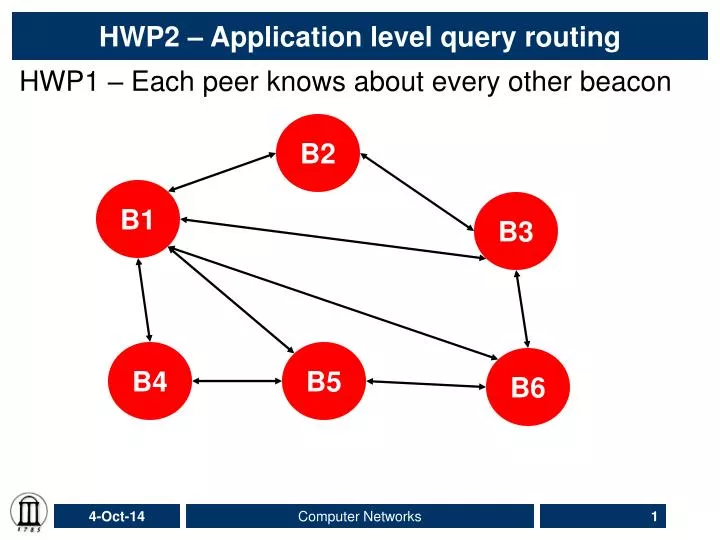
HWP2 – Application level query routing. HWP1 – Each peer knows about every other beacon. B2. B1. B3. B4. B5. B6. HWP2 – Query routing. searchget(searchkey, hopcount) Rget(host, port, key) Restrict each peer to maintain information about two other peers. B2. Scenario: 1. B1. B3. B4.

E N D
HWP2 – Application level query routing HWP1 – Each peer knows about every other beacon B2 B1 B3 B4 B5 B6 Computer Networks
HWP2 – Query routing • searchget(searchkey, hopcount) • Rget(host, port, key) • Restrict each peer to maintain information about two other peers B2 Scenario: 1 B1 B3 B4 B5 B6 Computer Networks
HWP2 – Distributed search • searchget(searchkey, hopcount) • Rget(host, port, key) • Restrict each peer to maintain information about two other peers B2 Scenario: 2 B1 B3 B4 B5 B6 Computer Networks
HWP2 – Distributed search • searchget(searchkey, hopcount) • Rget(host, port, key) B2 SRC Hop count=3 Scenario: 1 B1 B3 B4 B5 B6 DST Computer Networks
HWP2 – Distributed search • searchget(searchkey, hopcount) • Rget(host, port, key) B2 SRC Hop count=3 Scenario: 1 HC=1 B1 B3 HC=2 HC=2 HC=2 HC=0 B4 B5 B6 DST Computer Networks
HWP2 – Distributed search • searchget(searchkey, hopcount) • Rget(host, port, key) B2 SRC Hop count=3 Scenario: 2 B1 B3 B4 B5 B6 Computer Networks
Searchget • You will use controlled flooding to search for key • Rget • You will use routing technologies Computer Networks
Reference HWP1 solution • C source code will be available in the course web page (home works section) • Four threads • locatePeersSend • Continously sends identification every BEAT seconds on multicast port • Garbage collects clients that you haven’t heard in 3*BEAT seconds • locatePeersRecv • Receives multicast packets and adds to internal table • Sends ACK back – useful for RTT calculation • RTT • Receives ACK packets – compute RTT • serviceRequest • Services telnet clients for tuple service Computer Networks
Switching and Forwarding • Outline • Store-and-Forward Switches • Bridges and Extended LANs • Cell Switching • Segmentation and Reassembly Computer Networks
T3 T3 Switch T3 T3 STS-1 STS-1 Input Output ports ports Scalable Networks • Switch • forwards packets from input port to output port • port selected based on address in packet header • Advantages • cover large geographic area (tolerate latency) • support large numbers of hosts (scalable bandwidth) Computer Networks
Source Routing Computer Networks
0 Switch 1 3 1 2 Switch 2 2 3 1 5 11 0 Host A 7 0 Switch 3 1 3 4 Host B 2 Virtual Circuit Switching • Explicit connection setup (and tear-down) phase • Subsequence packets follow same circuit • Sometimes called connection-oriented model • Analogy: phone call • Each switch maintains a VC table Computer Networks
Host D Host E 0 Switch 1 Host F 3 1 Switch 2 2 Host C 2 3 1 0 Host A 0 Switch 3 Host B Host G 1 3 2 Host H Datagram Switching • No connection setup phase • Each packet forwarded independently • Sometimes called connectionless model • Analogy: postal system • Each switch maintains a forwarding (routing) table Computer Networks
Virtual Circuit Model • Typically wait full RTT for connection setup before sending first data packet. • While the connection request contains the full address for destination, each data packet contains only a small identifier, making the per-packet header overhead small. • If a switch or a link in a connection fails, the connection is broken and a new one needs to be established. • Connection setup provides an opportunity to reserve resources. Computer Networks
Datagram Model • There is no round trip time delay waitint for connection setup; a host can send data as soon as it is ready. • Source host has no way of knowing if the network is capable of delivering a packet or if the destination host is even up. • Since packets are treated independently, it is possible to route around link and node failures. • Since every packet must carry the full address of the destination, the overhead per packet is higher than for the connection-oriented model. Computer Networks
A B C Port 1 Bridge Port 2 Z X Y Bridges and Extended LANs • LANs have physical limitations (e.g., 2500m) • Connect two or more LANs with a bridge • accept and forward strategy • level 2 connection (does not add packet header) • Ethernet Switch = Bridge on Steroids Computer Networks
A B C Port 1 Bridge Port 2 X Y Z Learning Bridges • Do not forward when unnecessary • Maintain forwarding table • Learn table entries based on source address • Table is an optimization; need not be complete • Always forward broadcast frames Computer Networks
A B B3 C B5 D B7 K B2 E F B1 G H B6 B4 I J Spanning Tree Algorithm • Problem: loops • Bridges run a distributed spanning tree algorithm • select which bridges actively forward • developed by Radia Perlman • now IEEE 802.1 specification Computer Networks
Algorithm Overview • Each bridge has unique id (e.g., B1, B2, B3) • Select bridge with smallest id as root • Select bridge on each LAN closest to root as designated bridge (use id to break ties) • Each bridge forwards frames over each LAN for which it is the designated bridge A B B3 C B5 D B7 K B2 E F B1 G H B6 B4 I J Computer Networks
Algorithm Details • Bridges exchange configuration messages • id for bridge sending the message • id for what the sending bridge believes to be root bridge • distance (hops) from sending bridge to root bridge • Each bridge records current best configuration message for each port • Initially, each bridge believes it is the root Computer Networks
Algorithm Detail (cont) • When learn not root, stop generating config messages • in steady state, only root generates configuration messages • When learn not designated bridge, stop forwarding config messages • in steady state, only designated bridges forward config messages • Root continues to periodically send config messages • If any bridge does not receive config message after a period of time, it starts generating config messages claiming to be the root Computer Networks
Broadcast and Multicast • Forward all broadcast/multicast frames • current practice • Learn when no group members downstream • Accomplished by having each member of group G send a frame to bridge multicast address with G in source field Computer Networks
Limitations of Bridges • Do not scale • spanning tree algorithm does not scale • broadcast does not scale • Do not accommodate heterogeneity • Caution: beware of transparency Computer Networks
Cell Switching (ATM) • Connection-oriented packet-switched network • Used in both WAN and LAN settings • Signaling (connection setup) Protocol: Q.2931 • Specified by ATM forum • Packets are called cells • 5-byte header + 48-byte payload • Commonly transmitted over SONET • other physical layers possible Computer Networks
Variable vs Fixed-Length Packets • No Optimal Length • if small: high header-to-data overhead • if large: low utilization for small messages • Fixed-Length Easier to Switch in Hardware • simpler • enables parallelism Computer Networks
Big vs Small Packets • Small Improves Queue behavior • finer-grained pre-emption point for scheduling link • maximum packet = 4KB • link speed = 100Mbps • transmission time = 4096 x 8/100 = 327.68us • high priority packet may sit in the queue 327.68us • in contrast, 53 x 8/100 = 4.24us for ATM • near cut-through behavior • two 4KB packets arrive at same time • link idle for 327.68us while both arrive • at end of 327.68us, still have 8KB to transmit • in contrast, can transmit first cell after 4.24us • at end of 327.68us, just over 4KB left in queue Computer Networks
Big vs Small (cont) • Small Improves Latency (for voice) • voice digitally encoded at 64KBps (8-bit samples at 8KHz) • need full cell’s worth of samples before sending cell • example: 1000-byte cells implies 125ms per cell (too long) • smaller latency implies no need for echo cancellors • ATM Compromise: 48 bytes = (32+64)/2 Computer Networks
4 16 3 1 8 8 384 (48 bytes) GFC VPI VCI Type CLP HEC (CRC-8) Payload Cell Format • User-Network Interface (UNI) • host-to-switch format • GFC: Generic Flow Control (still being defined) • VCI: Virtual Circuit Identifier • VPI: Virtual Path Identifier • Type: management, congestion control, AAL5 (later) • CLPL Cell Loss Priority • HEC: Header Error Check (CRC-8) • Network-Network Interface (NNI) • switch-to-switch format • GFC becomes part of VPI field Computer Networks
Segmentation and Reassembly • ATM Adaptation Layer (AAL) • AAL 1 and 2 designed for applications that need guaranteed rate (e.g., voice, video) • AAL 3/4 designed for packet data • AAL 5 is an alternative standard for packet data AAL AAL … … A TM A TM Computer Networks
AAL 3/4 • Convergence Sublayer Protocol Data Unit (CS-PDU) • CPI: commerce part indicator (version field) • Btag/Etag:beginning and ending tag • BAsize: hint on amount of buffer space to allocate • Length: size of whole PDU Computer Networks
Cell Format • Type • BOM: beginning of message • COM: continuation of message • EOM end of message • SEQ: sequence of number • MID: message id • Length: number of bytes of PDU in this cell Computer Networks
AAL5 • CS-PDU Format • pad so trailer always falls at end of ATM cell • Length: size of PDU (data only) • CRC-32 (detects missing or misordered cells) • Cell Format • end-of-PDU bit in Type field of ATM header Computer Networks
Router Construction • Outline • Switched Fabrics • IP Routers • Extensible (Active) Routers Computer Networks
I/O bus CPU Interface 1 Interface 2 Interface 3 Main memory Workstation-Based • Aggregate bandwidth • 1/2 of the I/O bus bandwidth • capacity shared among all hosts connected to switch • example: 800Mbps bus can support 8 T3 ports • Packets-per-second • must be able to switch small packets • 100,000 packets-per-second is achievable • e.g., 64-byte packets implies 51.2Mbps Computer Networks
Input Output port port Output Input port port Fabric Output Input port port Output Input port port Switching Hardware • Design Goals • throughput (depends on traffic model) • scalability (a function of n) • Ports • circuit management (e.g., map VCIs, route datagrams) • buffering (input and/or output) • Fabric • as simple as possible • sometimes do buffering (internal) Computer Networks
Buffering • Wherever contention is possible • input port (contend for fabric) • internal (contend for output port) • output port (contend for link) • Head-of-Line Blocking • input buffering Computer Networks
Crossbar Switches Computer Networks
Inputs D D D D D D D D D D D D D D 1 2 3 4 Outputs Knockout Switch • Example crossbar • Concentrator • select l of n packets • Complexity: n2 Computer Networks
Shifter (a) Buffers Shifter (b) Buffers Shifter (c) Buffers Knockout Switch (cont) • Output Buffer Computer Networks
Self-Routing Fabrics • Banyan Network • constructed from simple 2 x 2 switching elements • self-routing header attached to each packet • elements arranged to route based on this header • no collisions if input packets sorted into ascending order • complexity: n log2 n Computer Networks
Self-Routing Fabrics (cont) • Batcher Network • switching elements sort two numbers • some elements sort into ascending (clear) • some elements sort into descending (shaded) • elements arranged to implement merge sort • complexity: n log22 n • Common Design: Batcher-Banyan Switch Computer Networks
High-Speed IP Router • Switch (possibly ATM) • Line Cards + Forwarding Engines • link interface • router lookup (input) • common IP path (input) • packet queue (output) • Network Processor • routing protocol(s) • exceptional cases Computer Networks
Routing software w/ router OS Line card (forwarding buffering) Routing CPU Buffer memory Line card (forwarding buffering) Line card (forwarding buffering) Line card (forwarding buffering) High-Speed Router Computer Networks
PC PC PC PC PC PC NI with uP NI with uP NI with uP NI with uP NI with uP NI with uP CPU CPU CPU CPU CPU CPU . . . . . . . . . . . . . . . . . . MEM MEM MEM MEM MEM MEM NI with uP NI with uP NI with uP NI with uP NI with uP NI with uP Crossbar Switch Alternative Design Computer Networks