Download
1 / 26
260 likes | 394 Views
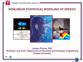
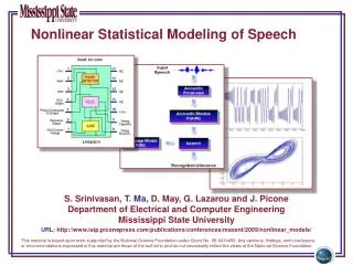
NONLINEAR STATISTICAL MODELING OF SPEECH. Joseph Picone, PhD Professor, Department of Electrical and Computer Engineering Mississippi State University. URL:. Abstract.

E N D
NONLINEAR STATISTICAL MODELING OF SPEECH Joseph Picone, PhD Professor, Department of Electrical and Computer Engineering Mississippi State University URL:
Abstract Statistical or machine-learning techniques, such as Hidden Markov models and Gaussian mixture models, have dominated the signal processing and pattern recognition literature for the past 25 years. However, such approaches are prone to overfitting and have problems with generalization. For example, delivering high performance on previously unseen noise conditions remains an elusive goal. In this presentation, we will review our recent work on applying principles of nonlinear statistical modeling to acoustic modeling in speech recognition. Our goal is to improve recognition performance in noisy environments. We will discuss the use of an extended feature vector containing features based on correlation dimension, correlation entropy and Lyapunov exponents. We will also introduce a new acoustic model based on a probabilistic mixture of autoregressive models. Experimental results are presented on the Aurora IV large vocabulary speech recognition task in which audio data from a variety of actual noise conditions were digitally added to the standard Wall Street Journal 5K closed-vocabulary task. We will show modest gains in performance can be achieved under matched conditions, but performance degraded under mismatched training conditions.
Fundamental Challenges: Generalization and Risk • Why research human language technology? • “Language is the preeminent trait of the human species.” • “I never met someone who wasn’t interested in language.” • “I decided to work on language because it seemed to be the hardest problem to solve.” • Some fundamental challenges: • Diversity of data, much of which defies simple mathematical descriptions or physical constraints (e.g., Internet data). • Too many unique problems to be solved (e.g., 6,000 language, billions of speakers, thousands of linguistic phenomena). • Generalization and risk are fundamental challenges (e.g., how much can we rely on sparse data sets to build high performance systems). • Underlying technology is applicable to many application domains: • Fatigue/stress detection, acoustic signatures (defense, homeland security); • EEG/EKG and many other biological signals (biomedical engineering); • Open source data mining, real-time event detection (national security). • Significant technology commercialization opportunities!
Speech Recognition Overview InputSpeech • Based on a noisy communication channel model in which the intended message is corrupted by a sequence of noisy models • Bayesian approach is most common: • Objective: minimize word error rate by maximizing P(W|A) • P(A|W): Acoustic Model • P(W): Language Model • P(A): Evidence (ignored) • Acoustic models use hidden Markov models with Gaussian mixtures. • P(W) is estimated using probabilisticN-gram models. • Parameters can be trained using generative (ML)or discriminative (e.g., MMIE, MCE, or MPE) approaches. AcousticFront-end Research Focus Acoustic ModelsP(A/W) Language ModelP(W) Search Recognized Utterance
Fundamental Challenges in Spontaneous Speech • Common phrases experience significant reduction (e.g., “Did you get” becomes “jyuge”). • Approximately 12% of phonemes and 1% of syllables are deleted. • Robustness to missing data is a critical element of any system. • Linguistic phenomena such as coarticulation produce significant overlap in the feature space. • Decreasing classification error rate requires increasing the amount of linguistic context. • Modern systems condition acoustic probabilities using units ranging from phones to multiword phrases.
Towards Nonlinear Acoustic Modeling • ARHMM: • autoregressive time series model for feature vectors integrated into an HMM framework • GMMs: • use multiple mixture components to accommodate modalities in the data; • rely on a feature vector to capture dynamics of the signal; • classification tends to perform poorly on unseen data. • Pro: directly models dynamics beyond1st and 2nd-order derivatives • Con: marginal improvements in performance at a much greater computational cost. • Chaotic Models: • capitalize on self-synchronization and limit cycle behavior.
Relevant Attributes of Nonlinear Systems • A PLL is a relatively simple, but very robust, nonlineardevice that uses negative feedback to match the frequency and phase of an input signal to a reference. • Our original goal was to build “phone detectors” that demonstrated similar properties to a PLL. • A strange attractor is a set of points or region which bounds the long-term, or steady-state behavior of a chaotic system. Systems can have multiple strange attractors, and the initial conditions determine which strange attractor is reached. • Our original goal was to build “chaotic” phone acoustic models that replaced conventional CDHMM phone models. • However, phonemes in spontaneous speech can be extremely short – 10 to30 ms durations are not uncommon. Also, some phonemes are transient in nature (e.g., stop consonants). This makes such modeling difficult. • In this talk, we will focus on two promising approaches: • Feature vectors using nonlinear dynamic invariants; • Acoustic models using Nonlinear Mixture Autoregressive HMMs.
Towards Improving Features for Speech Recognition InputSpeech • First attempt involved extended a standard speech recognition feature vector with some parameters that estimate the strength of the nonlinearities in the signal. • Direct modeling of the speech signal usingnonlinear dynamics has not been promising. • We were interested in a series of pilot experiments to understand the value of these features in various tasks such as speaker-independent recognition, where short-term spectral information is important, and speaker verification, where long-term spectral information is important. • Also used this testbed to tune variousparameters required in the calculation of these new features. • Investigated optimal ways to combine the features as well. AcousticFront-end Acoustic ModelsP(A/W) Language ModelP(W) Search Recognized Utterance
The Reconstructed Phase Space • Nonlinear invariants are computed from the phase space: • Signal amplitude is an observable of the system • Phase space is reconstructed from the observable • Invariants based on properties of the phase space • Reconstructed phase space (RPS): • time evolution of the system forms a path, or trajectory within the phase space; • the system’s attractor is the subset of the phase space to which the trajectory settles; • use SVD embedding to estimate the RPS(SVD reduction from 11 dimensions to 5). • Examples of an RPS for speech signals (phonemes): /ah/ /eh/ /m/ /sh/ /z/
Three Promising Nonlinear Invariants (D. May) • Correlation Dimension (Cdim): • quantifies attractor’s geometrical complexity by measuring self-similarity; • tends to be lower for fricatives and higher for vowels (not unlike other spectral measures such as the linear prediction order) . • Correlation Entropy (Cent): • measures the average rate of information production in a dynamic system; • tends to be low for nasals, and is less predictable for other sounds. • LyapunovExponent (): • measures the level of chaos in the reconstructed attractor; • tends to be low for nasals and vowels; high for unvoiced phones. Cdim = 0.84 Cent = 343 = -9.0 Cdim = 0.88 Cent = 666 = -7.7 /m/ /ah/ Cdim = 0.33 Cent = 623 = 795 /sh/
Continuous Speech Recognition Experiments • Evaluation: ETSI Aurora IV Distributed Speech Recognition (DSR) • Based on the Wall Street Journal corpus (moderate CPU requirements) • Digitally-added noise conditions at controlled SNRs • Baseline recognition system was the Aurora IV evaluation system (ISIP): • Features: industry-standard 39-dimension MFCC features • Acoustic Model: 4-mixture cross-word context-dependent triphones • Training: standard HMM approach (EM/BW/ML) • Decoding: one-best Viterbibeam search with a bigram 5K closed-set LM • Four feature combinations:
Experimental Results on Aurora IV • The contributions of each feature was analyzed as a function of the broad phonetic class. • A closed-set test was conducted on the training data. • The overall results were mixed and showed no consistent trend. • Two more extensive evaluations were conducted on Aurora IV: • Mismatched training: • Clean data (studio quality): • p < 0.001 are statistically significant.
Towards Improved Acoustic Modeling InputSpeech • Investigated a wide variety of nonlinearmodeling techniques including Kalmanfilters and particle filters with mixed results. • Focused on a technique that preservesthe benefits of autoregressive modeling,but adds a probabilistic component toallow modeling of nonlinearities. • Initially investigated this technique ondata involving artificially elongatedpronunciations of vowels to removeevent duration as a variable. • Techniques to extend these techniques to large-scale experiments on large vocabulary speech recognition tasks are underdevelopment. • The goal remains to achieve high performancerecognition on speech contaminated by noise not represented in the training database. AcousticFront-end Acoustic ModelsP(A/W) Language ModelP(W) Search Recognized Utterance
Mixture Autoregressive (MAR) Models (S. Srinivasan) • Define a weighted sum of autoregressive models (Wong and Li, 2000): • where, • εi: zero mean Gaussian with variance σj2 • “w.p. wi” : with probability wi • ai,j(j>0) : AR predictor coefficients • ai,0 : mean for the ith component • An AR filter of order 0 is equivalent to a Gaussian mixture model (GMM). • MFCCs routinely use 1st and 2nd order derivatives of the features to introduce some dynamic information into the HMM. • MAR can capture more information about dynamics using an AR model.
Integrating MAR into HMMs • Phonetic models in an HMM approach typically use a 3-state left-to-right model topology with a large number of mixture components (e.g., 128 mixtures for speech recognition and 1024 mixtures for speaker verification). • Dynamics are captured in the feature vector and through the state transition probabilities. • Observation probabilities tend to dominate. • MAR-HMM uses a probabilistic MAR model in which the weights are estimated using the EM algorithm. • In our work we have extended the scalar MAR model to handle feature vectors by using a single weight estimated by summing the likelihoods across all scalar components.
Experimental Results on Sustained Phones • MAR-HMM was initially evaluated on a pilot corpus of sustained vowels that was developed to prototype nonlinear algorithms. • Results are shown in terms of % accuracy and the number of parameters (in parentheses). • For the same number of parameters, MAR-HMM has a slight advantage. • MAR performance saturates as the number of parameters increases. • Assumption that features are uncorrelated during MAR training is invalid., particularly for delta features. This typically causes problems for both GMMs and MAR, but it seems to impact MAR-HMM more significantly. • Results on continuous speech recognition have not been promising and are the subject of further research.
Summary • Introduced two attempts to add nonlinear statistical models to conventional hidden Markov model (HMM) speech recognition systems. • Demonstrated slight improvements in performance on clean data, but did not achieve our overall goal of improving performance on unseen noisy data. • We are continuing to examine alternate acoustic modeling techniques and are pursuing an alternative known as a linear dynamic model. However, preliminary results are similarly mixed. • We have seen similar modest improvements in speaker identification and verification performance. Here, we overcome the problem of a lack of samples since features are extracted across an entire utterance. However, deconvolving short-term spectral variations and long-term speaker characteristics remains a challenge. • Future directions will include non-Bayesian statistical models.
Brief Bibliography of Related Research • D. May, Nonlinear Dynamic Invariants For Continuous Speech Recognition, M.S. Thesis, Department of Electrical and Computer Engineering, Mississippi State University, May 2008. • S. Srinivasan, T. Ma, D. May, G. Lazarou and J. Picone, "Nonlinear Mixture Autoregressive Hidden Markov Models For Speech Recognition,"Proceedings of the International Conference on Spoken Language Processing, pp. 960-963, Brisbane, Australia, September 2008. • T. Ma, S. Srinivasan, D. May, G. Lazarou and J. Picone, "Robust Speech Recognition Using Linear Dynamic Models," submitted to INTERSPEECH, Brisbane, Australia, September 2008. • S. Prasad, S. Srinivasan, M. Pannuri, G. Lazarou and J. Picone, "Nonlinear Dynamical Invariants for Speech Recognition,"Proceedings of the International Conference on Spoken Language Processing, pp. 2518-2521, Pittsburgh, Pennsylvania, USA, September 2006. • Y. Ephraim and W.J.J. Roberts, “Revisiting Autoregressive Hidden Markov Modeling of Speech Signals,” IEEE Signal Processing Letters, vol. 12, no. 2, pp. 166-169, Feb. 2005. • H. Kantz and T. Schreiber, Nonlinear Time Series Analysis, Cambridge University Press, New York, New York, USA, 2003.
Appendix: Correlation Integral • The correlation integral quantifies how completely theattractor fills the phase space by measuring the densityof the points close to the attractor’s trajectory, and averaging this density over the entire attractor. • Computed using the following steps: • consider a window of data (30 ms) centered around a frame (10 ms); • choose a neighborhood radius, ε, and center a hypersphere with this radius on the initial point of the attractor (ε = 2.3); • count the number of points within the hypersphere; • move the center of the hyper-sphere to the next point along the trajectory of the attractor and repeat step 2; • compute the average of the number of points falling within the hypersphere over the entire attractor. • Mathematically, this is expressed by: • nmin is a correction factor (Theiler) which reduces the negative effects of temporal correlations by skipping points which are temporally close. /ah/
Appendix: Correlation Dimension • The correlation dimension captures the power-law relation between the correlation integral of the attractor and the neighborhood radius of the hypersphere as the number of points on the attractor approaches infinity and ε becomes very small. • The relationship between the correlation integral and correlation dimension is (for small ε): • The correlation dimension is computed using the correlation integral: • Our approach is to choose a minimum value for ε via tuning (εmin = 0.2), choose a range for ε in this neighborhood (0.2 ε 2.3), a resolution for this range (εstep = 0.1), compute the correlation integral for ε, and finally computing the slope using a smoothing approach (regression). • Theoretically, this should be a close approximation to the fractal dimension.
Appendix: Correlation Entropy • A measure of dynamic systems is the rate at which new information is being produced as a function of time. • Each new observation of a dynamic system potentially contributes new information to this system, and the average quantity of this new information is referred to as the metric, or Kolmogorov entropy. • For reconstructed phase spaces, it is easier to compute the second-order metric entropy, K2, because it is related to the correlation integral: • where D is the fractal dimension of the reconstructed attractor, ε is the neighborhood radius, m and are the number of embedding dimensions and time delay, respectively, used for phase space reconstruction. • From this relation, an expression for K2 can be derived: • We compute the (log) correlation integral for an RPS in m=5 and m+1=6 dimensions. ε is minimized via tuning (εmin=2.3). K2 is the ratio scaled by (1/).
Appendix: Lyapunov Exponents • Describe the relative behavior of neighboring trajectorieswithin an attractor and quantify the level of chaos. • Determine the level of predictability of the system byanalyzing trajectories that are in close proximity and measuring the change in this proximity as time evolves. • The separation between two trajectories with close initial points after Nevolution stepscan be represented by: • High-level overview of our approach: • Reconstruct phase space from the original time-series. • Select a point on the reconstructed attractor. • Find a set of nearest neighbors to . • Measure the separation between and its neighbors as time evolves. • Compute the local Lyapunov exponent from separation measurements. • Repeat steps 2 though 5 for each of the reconstructed attractor. • Compute average Lyapunov exponent from the local exponents.
Appendix: Lyapunov Exponents (Cont.) • Mathematically, the Lyapunov exponent is represented by: • The algorithm makes one pass over the attractor, starting from the first embedded state, advancing by the defined step size for a maximum of the defined number of steps. • In our experiments, the number of steps was sufficientlylarge to include the entire attractor. • At each step, we find the nearest N neighbors and store these neighbors. We then step the state and its neighbors according to the step size, and again store the evolved neighbors. • Next we group the set of original neighbors into subgroups. If any of these neighbors are on the same local trajectory, we group them into the same subgroup. We then group the evolved neighbors into the same groups as their originators and take the average of each subgroup and store these in a matrix. • At this point, we have 2 matrices: the average nearest neighbor subgroup matrix, and the average evolved nearest neighbor subgroup matrix.
Appendix: Lyapunov Exponents (Cont.) • We compute a trajectory matrix based on the singular values of each of these matrices which defines the direction of all the neighboring trajectories represented by the neighbor subgroups. • From the trajectory matrix, we can compute the Lyapunov spectrum by taking the QR decomposition of the trajectory matrix, and taking the log of the diagonal values for the upper-triangular matrix (R). • The Lyapunov exponent is (typically) taken as the maximum Lyapunov spectrum value. • We repeat the process above across the whole attractorand average the Lyapunov exponents to arrive at our finalexponent. • The parameters which must be chosen for this algorithm include the size of the neighborhood (ε= 25), the number of time evolution steps (5samples), and the number of embedding dimensions (m= 5) for SVD embedding. These parameters are typically found experimentally.
Appendix: Major ISIP Milestones • 1994: Founded the Institute for Signal and Information Processing (ISIP) • 1995: Human listening benchmarks established for the DARPA speech program • 1997: DoD funds the initial development of our public domain speech recognition system • 1997: Syllable-based speech recognition • 1998: NSF CARE award for Internet-Accessible Speech Recognition Technology • 1998: First large-vocabulary speech recognition application of Support Vector Machines • 1999: First release of high-quality SWB transcriptions and segmentations • 2000: First participation in the annual DARPA evaluations (only university site to participate) • 2000: NSF funds a multi-university collaboration on integrating speech and natural language • 2001: Demonstrated the small impact of transcription errors on HMM training • 2002: First viable application of Relevance Vector Machines to speech recognition • 2002: Distribution of Aurora toolkit • 2002: Evolution of ISIP into the Institute for Intelligent Electronic Systems • 2002: the “Crazy Joe” commercial becomes the most widely viewed ISIP document • 2003: IIES joins the Center for Advanced Vehicular Systems • 2004: NSF funds nonlinear statistical modeling research and supports the development of speaker verification technology • 2004: ISIP’s first speaker verification system • 2005: ISIP’s first dialog system based on our port to the DARPA Communicator system • 2006: Automatic detection of fatigue • 2007: Integration of nonlinear features into a speech recognition front end • 2008: ISIP’s first keyword search system • 2008: Nonlinear mixture autoregressive models for speech recognition • 2008: Linear dynamic models for speech recognition • 2009: Launch of our first commercial web site and associated business venture…
Biography Joseph Picone received his Ph.D. in Electrical Engineering in 1983 from the Illinois Institute of Technology. He is currently a Professor in the Department of Electrical and Computer Engineering at Mississippi State University. He recently completed a three-year sabbatical at the Department of Defense where he directed human language technology research and development. His primary research interests are currently machine learning approaches to acoustic modeling in speech recognition. For over 25 years he has conducted research on many aspects of digital speech and signal processing. He has also been a long-term advocate of open source technology, delivering one of the first state-of-the-art open source speech recognition systems, and maintaining one of the more comprehensive web sites related to signal processing. His research group is known for producing many innovative educational materials that have increased access to the field. Dr. Picone has previously been employed by Texas Instruments and AT&T Bell Laboratories, including a two-year assignment in Japan establishing Texas Instruments’ first international research center. He is a Senior Member of the IEEE and has been active in several professional societies related to human language technology. He has authored numerous papers on the subject and holds 8 patents.