9. Two Functions of Two Random Variables

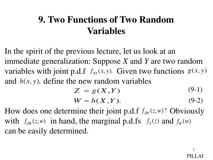
1. 9. Two Functions of Two Random Variables In the spirit of the previous lecture, let us look at an immediate generalization: Suppose X and Y are two random variables with joint p.d.f Given two functions and define the new random variables How does one determine their joint p.d.f Obviously with in hand, the marginal p.d.fs and can be easily determined. (9-1) (9-2) PILLAI

2. Fig. 9.1 The procedure is the same as that in (8-3). In fact for given z and w, where is the region in the xy plane such that the inequalities and are simultaneously satisfied. We illustrate this technique in the next example. (9-3) PILLAI

3. Example 9.1: Suppose X and Y are independent uniformly distributed random variables in the interval Define Determine Solution: Obviously both w and z vary in the interval Thus We must consider two cases: and since they give rise to different regions for (see Figs. 9.2 (a)-(b)). (9-4) (9-5) Fig. 9.2 PILLAI

4. For from Fig. 9.2 (a), the region is represented by the doubly shaded area. Thus and for from Fig. 9.2 (b), we obtain With we obtain Thus (9-6) (9-7) (9-8) (9-9) (9-10) PILLAI

5. From (9-10), we also obtain and If and are continuous and differentiable functions, then as in the case of one random variable (see (5-30)) it is possible to develop a formula to obtain the joint p.d.f directly. Towards this, consider the equations For a given point (z,w), equation (9-13) can have many solutions. Let us say (9-11) (9-12) (9-13) PILLAI

6. (b) (a) represent these multiple solutions such that (see Fig. 9.3) (9-14) Fig. 9.3 Consider the problem of evaluating the probability (9-15) PILLAI

7. (a) (b) Using (7-9) we can rewrite (9-15) as But to translate this probability in terms of we need to evaluate the equivalent region for in the xy plane. Towards this referring to Fig. 9.4, we observe that the point A with coordinates (z,w) gets mapped onto the point with coordinates (as well as to other points as in Fig. 9.3(b)). As z changes to to point B in Fig. 9.4 (a), let represent its image in the xy plane. Similarly as w changes to to C, let represent its image in the xy plane. (9-16) Fig. 9.4 PILLAI

8. Finally D goes to and represents the equivalent parallelogram in the XY plane with area Referring back to Fig. 9.3, the probability in (9-16) can be alternatively expressed as Equating (9-16) and (9-17) we obtain To simplify (9-18), we need to evaluate the area of the parallelograms in Fig. 9.3 (b) in terms of Towards this, let and denote the inverse transformation in (9-14), so that (9-17) (9-18) (9-19) PILLAI

9. As the point (z,w) goes to the point the point and the point Hence the respective x and y coordinates of are given by and Similarly those of are given by The area of the parallelogram in Fig. 9.4 (b) is given by (9-20) (9-21) (9-22) (9-23) PILLAI

10. But from Fig. 9.4 (b), and (9-20) - (9-22) so that and The right side of (9-27) represents the Jacobian of the transformation in (9-19). Thus (9-24) (9-25) (9-26) (9-27) PILLAI

11. (9-28) Substituting (9-27) - (9-28) into (9-18), we get since where represents the Jacobian of the original transformation in (9-13) given by (9-29) (9-30) (9-31) PILLAI

12. Next we shall illustrate the usefulness of the formula in (9-29) through various examples: Example 9.2: Suppose X and Y are zero mean independent Gaussian r.vs with common variance Define where Obtain Solution: Here Since if is a solution pair so is From (9-33) (9-32) (9-33) (9-34) PILLAI

13. Substituting this into z, we get and Thus there are two solution sets We can use (9-35) - (9-37) to obtain From (9-28) so that (9-35) (9-36) (9-37) (9-38) (9-39) PILLAI

14. We can also compute using (9-31). From (9-33), Notice that agreeing with (9-30). Substituting (9-37) and (9-39) or (9-40) into (9-29), we get Thus which represents a Rayleigh r.v with parameter and (9-40) (9-41) (9-42) (9-43) PILLAI

15. which represents a uniform r.v in the interval Moreover by direct computation implying that Z and W are independent. We summarize these results in the following statement: If X and Y are zero mean independent Gaussian random variables with common variance, then has a Rayleigh distribution and has a uniform distribution. Moreover these two derived r.vs are statistically independent. Alternatively, with X and Y as independent zero mean r.vs as in (9-32), X + jY represents a complex Gaussian r.v. But where Z and W are as in (9-33), except that for (9-45) to hold good on the entire complex plane we must have and hence it follows that the magnitude and phase of (9-44) (9-45) PILLAI

16. a complex Gaussian r.v are independent with Rayleigh and uniform distributions ~ respectively. The statistical independence of these derived r.vs is an interesting observation. Example 9.3: Let X and Y be independent exponential random variables with common parameter . Define U = X + Y, V = X - Y. Find the joint and marginal p.d.f of U and V. Solution: It is given that Now since u = x + y, v = x - y, always and there is only one solution given by Moreover the Jacobian of the transformation is given by (9-46) (9-47) PILLAI

17. and hence represents the joint p.d.f of U and V. This gives and Notice that in this case the r.vs U and V are not independent. As we show below, the general transformation formula in (9-29) making use of two functions can be made useful even when only one function is specified. (9-48) (9-49) (9-50) PILLAI

18. Auxiliary Variables: Suppose where X and Y are two random variables. To determine by making use of the above formulation in (9-29), we can define an auxiliary variable and the p.d.f of Z can be obtained from by proper integration. Example 9.4: Suppose Z = X + Y and let W = Y so that the transformation is one-to-one and the solution is given by (9-51) (9-52) PILLAI

19. The Jacobian of the transformation is given by and hence or which agrees with (8.7). Note that (9-53) reduces to the convolution of and if X and Y are independent random variables. Next, we consider a less trivial example. Example 9.5: Let  and  be independent. Define (9-53) (9-54) PILLAI

20. Find the density function of Z. Solution: We can make use of the auxiliary variable W = Y in this case. This gives the only solution to be and using (9-28) Substituting (9-55) - (9-57) into (9-29), we obtain (9-55) (9-56) (9-57) (9-58) PILLAI

21. and Let so that Notice that as w varies from 0 to 1, u varies from to Using this in (9-59), we get which represents a zero mean Gaussian r.v with unit variance. Thus  Equation (9-54) can be used as a practical procedure to generate Gaussian random variables from two independent uniformly distributed random sequences. (9-59) (9-60) PILLAI

22. Example 9.6 : Let X and Y be independent identically distributed Geometric random variables with (a) Show that min (X , Y ) and X – Y are independent random variables. (b) Show that min (X , Y ) and max (X , Y ) –min (X , Y ) are also independent random variables. Solution: (a) Let Z = min (X , Y ) , and W = X – Y. Note that Z takes only nonnegative values while W takes both positive, zero and negative values We have P(Z = m, W = n) = P{min (X , Y ) = m, X – Y = n}. But Thus (9-61) (9-62) PILLAI

23. (9-63) represents the joint probability mass function of the random variables Z and W. Also Thus Z represents a Geometric random variable since and (9-64) PILLAI

24. (9-65) Note that establishing the independence of the random variables Z and W. The independence of X – Y and min (X , Y ) when X and Y are independent Geometric random variables is an interesting observation. (b) Let Z = min (X , Y ) , R = max (X , Y ) – min (X , Y ). In this case both Z and R take nonnegative integer values Proceeding as in (9-62)-(9-63) we get (9-66) (9-67) PILLAI

25. (9-68) Eq. (9-68) represents the joint probability mass function of Z and R in (9-67). From (9-68), (9-69) PILLAI

26. and From (9-68)-(9-70), we get which proves the independence of the random variables Z and R defined in (9-67) as well. (9-70) (9-71) PILLAI