Download
1 / 19
190 likes | 374 Views
Two Random Variables. W&W, Chapter 5. Joint Distributions. So far we have been talking about the probability of a single variable, or a variable conditional on another. We often want to determine the joint probability of two variables, such as X and Y.

E N D
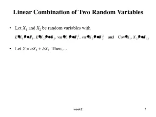
Two Random Variables W&W, Chapter 5
Joint Distributions So far we have been talking about the probability of a single variable, or a variable conditional on another. We often want to determine the joint probability of two variables, such as X and Y. Suppose we are able to determine the following information for education (X) and age (Y) for all U.S. citizens based on the census.
Joint Distributions Each cell is the relative frequency (f/N). We can define the joint probability distribution as: p(x,y) = Pr(X=x and Y=y) Example: what is the probability of getting a 30 year old college graduate?
Joint Distributions p(x,y) = Pr(X=3 and Y=30) = .07 We can see that: p(x) = y p(x,y) p(x=1) = .03 + .06 + .10 = .19
Marginal Probability We call this the marginal probability because it is calculated by summing across rows or columns and is thus reported in the margins of the table. We can calculate this for our entire table.
Independence Two random variables X and Y are independent if the events (X=x) and (Y=y) are independent, or: p(x,y) = p(x)p(y) for all x and y Note that this is similar to Event E is independent of F if: Pr(E and F) = Pr(E)Pr(F) Eq. 3-21
Example Are education and age independent? Start with the upper left hand cell: p(x,y) = .01 p(x) = .08 p(y) = .29 We can see they are not independent because (.08)(.29)=.0232, which is not equal to .01.
Independence In a table like this, if X and Y are independent, then the rows of the table p(x,y) will be proportional and so will the columns (see Example 5-1, page 158).
Covariance It is useful to know how two variables vary together, or how they co-vary. We begin with the familiar concept of variance (E is expectation). 2 = E(x- )2 = (x- )2 p(x) X,Y = Covariance of X and Y = E(X - X)(Y - Y) = (X - X)(Y - Y)p(x,y)
Covariance Let’s calculate the covariance for education (X) and age (Y). First we need to calculate the mean for X and Y: X = xp(x) = (0)(.08)+(1)(.19)+(2)(.54)+(3)(.19)=1.84 Y = yp(y) = (30)(.29)+(45)(.37)+(70)(.34)=49.15 Now calculate each value in the table minus its mean (for X and Y), multiplied by the joint probability!
Covariance X,Y = (X - X)(Y - Y)p(x,y) = (0-1.84)(30-49.15)(.01) + (0-1.84)(45-49.15)(.02) + (0-1.84)(70-49.15)(.05) + (1-1.84)(30-49.15)(.03) + (1-1.84)(45-49.15)(.06) + (1-1.84)(70-49.15)(.10) + (2-1.84)(30-49.15)(.18) + (2-1.84)(45-49.15)(.21) + (2-1.84)(70-49.15)(.15) + (3-1.84)(30-49.15)(.07) + (3-1.84)(45-49.15)(.08) + (3-1.84)(70-49.15)(.04) = -3.636
Covariance The covariance is negative, which tells us that as age increases, education decreases (and vice versa). It is negative because when one variable is above its mean, the other is below its mean on average. We can calculate covariance alternatively as X,Y = E(XY) - X Y = (xy)p(x,y) - X Y
Covariance and Independence If X and Y are independent, then they are uncorrelated, or their covariance is zero: X,Y = 0 The value for covariance depends on the units in which X and Y are measured. If X, for example, were measured in inches instead of feet, each X deviation and hence X,Y itself would increase by 12 times.
Correlation We can calculate the correlation instead: = X,Y X Y Correlation is independent of the scale it is measured in, and is always bounded: -1 1
Correlation A perfect positive correlation (=1); all x,y coordinate points will fall on a straight line with positive slope. A perfect negative correlation (=-1); all x,y coordinate points will fall on a straight line with negative slope. A correlation of zero indicates no relationship between X and Y (or independence!). Positive correlations (as X increases, Y increases) Negative correlations (as X increases, Y decreases)
Example of Correlation Calculate the correlation between education and age: = X,Y= -3.636 X Y (.8212)(16.14) = -0.2743
Interpretation There is a weak, negative correlation between education and age, which means that older people have less education. Later on we will learn how to conduct a hypothesis test to determine if is significantly different from zero.