Support Vector Machines

1. Support Vector Machines Reminder of perceptron Large-margin linear classifier Non-separable case

2. Linearly separable case Every vector in the grey region is a solution vector. The region is called the “solution region”. A vector in the middle looks better. We can impose conditions to select it.

3. Gradient descent procedure

4. Perceptron Y(a) is the set of samples mis-classified by a. When Y(a) is empty, define J(a)=0. Because aty <0 when yi is misclassified, J(a) is non-negative. The gradient is simple: The update rule is: Learning rate

5. Perceptron

6. Perceptron

7. Perceptron The perceptron adjusts a only according to misclassified samples; correctly classified samples are ignored. The final a is a linear combination of the training points. To have good testing-sample performance, a large set of training samples is needed; however, it is almost certain that a large set of training samples is not linearly separable. In the case of linearly non-separable, the iteration doesn’t stop. To make sure it converges, we can let η(k)  0 as k∞. However, how to choose the rate of change?

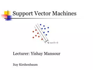
8. Large-margin linear classifier • Let’s assume the linearly separable case. • The optimal separating hyperplane separates the two classes and maximizes the distance to the closest point. f(x)=wtx+w0 • Unique solution • Better test sample performance

9. Large-margin linear classifier • {x1, ..., xn}: our training dataset in d-dimension • yiÎ {1,-1}: class label • Our goal: Among all f(x) such that • Find the optimal separating hyperplane  • Find the largest margin M,

10. Large-margin linear classifier • The border is M away from the hyperplane. M is called “margin”. • Drop the ||β||=1 requirement, Let M=1 / ||β||, then the easier version is:

11. Large-margin linear classifier

12. Non-separable case • When two classes are not linearly separable, allow slack variables for the points on the wrong side of the border:

13. Non-separable case • The optimization problem becomes: • ξ=0 when the point is on the correct side of the margin; • ξ>1 when the point passes the hyperplane to the wrong side; • 0<ξ<1 when the point is in the margin but still on the correct side.

14. Non-separable case • When a point is outside the boundary, ξ=0. It doesn’t play a big role in determining the boundary ---- not forcing any special class of distribution.

15. Computation • equivalent • C replaces the constant. • For separable case, C=∞.

16. Computation • A quadratic programming problem. The Lagrange function is: • Take derivatives of β, β0, ξi, set to zero: • And positivity constraints:

17. Computation • Substitute the three lower equations into the top one, the Lagrangian dual objective function: • Karush-Kuhn-Tucker conditions include

18. Computation • From , The solution of β has the form: • Non-zero coefficients only for those points i for which • These are called “support vectors”. • Some will lie on the edge of the margin • the remainder have , They are on the wrong side of the margin.

19. Computation

20. Computation • Smaller C. 85% of the points are support points.

21. Support Vector Machines • Enlarge the feature space to make the procedure more flexible. • Basis functions • Use the same procedure to construct SV classifier • The decision is made by

22. SVM • Recall in linear space: • With new basis:

23. SVM When domain knowledge is available, sometimes we could use explicit transformations. But often we cannot.

24. SVM • h(x) is involved ONLY in the form of inner product! • So as long as we define the kernel function • Which computes the inner product in the transformed space, we don’t need to know what h(x) itself is! “Kernel trick” • Some commonly used Kernels:

25. SVM • Recall αi=0 for non-support vectors, f(x) depends only on the support vectors.

26. SVM • K(x,x’) can be seen as a similarity measure between x and x’. • The decision is made essentially by a weighted sum of similarity of the object to all the support vectors.

27. SVM

28. SVM Bayes error: 0.029 When noise features are present, SVM suffered from not being able to concentrate on a subspace - all terms of the form 2XjXj′ are given equal weight

29. SVM • How to select kernel and parameters ? • Domain knowledge. • How complex should the space partition be? • Should the surface be smooth? • Compare the models by their approximate testing error rate cross-validation • - Fit data using multiple kernels/parameters • - Estimate error rate for each setting • - Select the best-performing one • Parameter optimization methods