Download
1 / 35
380 likes | 507 Views
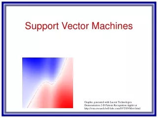
Support Vector Machines. Part I. Introduction Supervised learning Input/output and hyperplanes Support vectors Optimisation Key ideas: Input space & feature space Kernels Overfitting. Part II. „Fast and accurate Part-of-Speech Tagging: The SVM Approach revisited“

E N D
Part I Introduction • Supervised learning • Input/output and hyperplanes • Support vectors • Optimisation • Key ideas: • Input space & feature space • Kernels • Overfitting
Part II „Fast and accurate Part-of-Speech Tagging: The SVM Approach revisited“ (Jesús Giménez and Lluís Màrquez) • Problem Setting • Experiments, Results • Conclusion
1. Supervised Learning Learning by examples • Training set: pairs of input data labelled with output e.g. input: word & output: tag <word/tag> • Target function: mapping from input data to output, i.e. classifying <word> correctly as <tag> • Task: approximate this mapping = solution/decision function
1. Supervised Learning • Algorithm may select set of possible solutions = hypothesis space If the hypotheses,i.e. the output is : - binary binary classification task - finite multiclass classific. task - real-valued regression • Correctly classifying new data = generalisation
Support Vector Machines (SVMs) Hypothesis Space of linear functions („linear separator“) Training data: xn (n-dimensional vectors) Labels/classes: di (i different classes) Training Set: L = x £d = {(x1,d1),...,(xm,dm)} = {(xm,dm) / m=1,...M} Binary classification: Function f, Input xm if f(xm) > 0 if f(xm) < 0 positive class negative class d = +1 d = -1
2. SVM = Linear Separator • f(x) separates instances = hyperplane H H = H(w,b) = {x 2 Rn / wTx + b = 0} with w2 Rn and a bias b2 R • ForwTx + b ¸ +1, dm = +1 wTx + b · -1, dm = -1 • !dm * (wTx + b) ¸ 1 (normalised combined constraint)
3. Margin of Separation • Geometric margin r between x and H: r = (wTx + b) / ║w║ • Margin of Separation μL: μL(w,b) = minm=1,...,M ( |wTxm+b| / ║w║ )
μ μ H H
3. Margin of Separation The larger μ the more robust is H If μ is max in all directions then there exits pos. and neg. instances exactly on μ. Support Vectors (of H to L) • norm. distance rpos of support vectors from H: 1 / ||w|| • norm. distance rneg of support vectors from H: -1 / ||w||
4. Optimisation • Binary classification = „finding hyperplane that separates pos. & neg. instances“ (decision function) finding optimal hyperplane ! • No instances in (2 / ║w║) - space around H : maximise (2 / ║w║)
4. Optimisation • i.e. minimse (0.5 * wT * w) • satisfying the constraint dm * (wTx + b) ¸ 1 • How?
4. Lagrange Multiplier • Calculate ‚saddle point‘ of a function which has to satisfy a certain constraint: • Introduce (pos. & real-valued) and minimise function J Q() = J(w,b,) , dm * (wTx + b) ¸ 1 such that J(w*,) · J(w*,*) · J(w,*) • Solve and find optimal w
4. Lagrange Multiplier • Optimal w is a linear combination of trainings set L w = (m=1...M)m * dm * xm • but >0 only for dm * (wTxm + b) – 1=0, ie. for support vectors • optimal w is a linear combination of support vectors of L
4. Lagrange Multiplier • Q() : = 0.5wTw - (m=1,..M)m * (dm *(wTxm+ b)–1) = -0.5 * (m=1...M) (n=1...M)mn * dmdn * (xm)Txn + (m=1...M)m (only uses dot/scalar product in equation)
5. a) Feature Space If not linearly separable (e.g. XOR in 2D): Project to higher dimensional space = feature space : Rn RN; n lower dim, N higher dim Input space Rn, feature space RN
5. a) Feature Space Instead of L = {(xm,dm) / m=1,...M} L = {((xm),dm) / m=1,...M} Also for optimisation problem: Q() = -0.5 * mn * dmdn * ((xm)T (xn)) + m (Only dot product <(xm)T(xn)> !)
5. b) Kernel Functions • When : Rn RN then Kernel K : Rn£ Rn R dot products: K(x1, x2) = <(x1),(x2)> • Find K with least complex k, e.g. K(x,y) = k(xT,y)
5. b) Kernel Functions E.g. : R2 R4 : (x) = (x1, x2) (x) = (x12, x1*x2, x2*x1, x22) k(xT,y) = ?
6. Overfitting • w becomes too complex, data is modelled too closely • Allow for errors (data is noisy anyway) otherwise generalisation becomes poor • Soft margin:σ = 0.5wTw + C * ξ • New constraint on function: dm * (wTx + b) – (1- ξ) ¸ 0 = dm * (wTx + b) ¸ 1- ξ
Part II „Fast and accurate Part-of-Speech Tagging: The SVM Approach revisited“ (Jesús Giménez and Lluís Màrquez) • Problem Setting • Experiments, Results • Conclusion
1. Problem Setting • Tagging is multiclass classification task binarise by training an SVM for each class : • learn to distinguish between current class (i.e. <tag>) and the rest • Restrict classes/tags by using lexicon and use only other possible classes/tags as negative instances for current • When tagging, choose most confident tag out of all binary SVM predictions for <word> e.g. tag with greatest distance to separator
1. Problem Setting • Coding of features
1. Problem Setting • Evaluate to binary features: e.g. bigram: „previous_word_is_XXX“ = true/false • Context set to seven-token-window • When tagging, right-hand-tags are not yet known „ambiguity class“ = tag out of possible combinations („maybe“) • Only need to include explicit n-grams when linear kernels are used i.e. higher dim. Vector or higher dim. Kernel
2. Experiments • Corpus: Penn Treebank III (1,17 million words) • Corpus divided in: • Training set (60%) • Validation, i.e. parameter optimisation (20%) • Test set (20%) • Tagset with 48 tags, only 34 used as in 1.,i.e. 34 SVMs; rest unambiguos
2. Experiments • Linear vs Polynomial Kernels • test various kernels acc. to degree d • each with default C-parameter • features filtered by number of occurrences n
2. Experiments • For feature set 1, degree 2 pol. Kernel is best • higher degrees lead to overfitting: more support vectors, less accuracy • For feature set 2 (incl. n-grams), linear Kernel is best, even better than degree 2 Kernel • less support vectors (sparse) and 3 times faster ! • Preferable to extend feature set with n-grams and use linear Kernel
2. Experiments - Results • Linear Kernel • greedy left-to-right tagging with no optimisation on sentence level • Closed vocabulary assumption Performance in accuracy (compared to state-of-the-art HMM-based tagger TnT)
2. Experiments • Include unknown words: • ambiguous word with all open-word classes as possible tags (18) • use feature template, e.g.: • All Upper/Lower Case: yes/no • Contains Capital letters: yes/no • Contains a period/number... : yes/no • Suffixes: s1, s1s2, s1s2s3,... • AND all features for known words
2. Experiments - Results • SVMtagger+, implemented in Perl: • tagging speed of 1335 words/sec • maybe faster in C++ ?! • TnT: • speed of 50000 words/sec
3. Conclusion • State-of-the-art NLP-tool suited for real applications • represents a good balance of: • simplicity • flexibility (not domain-specific) • high performance • efficiency
3. Future Work • Experiment with and improve learning model for unknown words • Implement in C++ • Include probabilities of the whole sentence tag sequence in tagging scheme • Simplify model, i.e. decision function / hyperplane based on w • (accuracy is hardly worse with up to 70% of w‘s dimensions discarded – how?)