Download
1 / 24
240 likes | 380 Views
Bayesian Deconvolution of Belowground Ecosystem Processes Kiona Ogle University of Wyoming Departments of Botany & Statistics. Ecosystem Processes. Emphasis on aboveground. What about belowground?. Biogeochemical Cycles. H 2 0. N. H 2 0. N. H 2 0. C. C. P. H 2 0. N. H 2 0. N.

E N D
Bayesian Deconvolution of Belowground Ecosystem Processes Kiona Ogle University of Wyoming Departments of Botany & Statistics
Ecosystem Processes Emphasis on aboveground What about belowground?
Biogeochemical Cycles H20 N H20 N H20 C C P
H20 N H20 N H20 C C P Biogeochemical Cycles Belowground system is critical to understanding and forecasting whole-ecosystem behavior
Deconvolution of Belowground Processes • The water cycle • Partitioning plant water sources • The carbon cycle • Partitioning soil respiration • Data-model assimilation • Diverse data sources • Stable isotopes • Bayesian deconvolution framework Today’s example
Challenges • Patitioning sources of CO2 fluxes • Systems: soils & ecosystems • Sources: autotrophs vs. heterotrophs • Source contributions wrt soils: • By soil depth (including litter) • By species or functional group (autotrophs) • Spatial variability • Temporal dynamics • Environmental drivers
CO2 CO2 CO2 ?? ?? ?? ?? Relative contributions of C3 roots (shrub), C4 roots (grass), and heterotrophs (soil & litter)? From where in the soil is CO2 coming from? Partitioning Soil Respiration How does pulse precipitation affect sources of respired CO2? CO2
Bayesian Deconvolution Approach • Integrate multiple sources of information • Diverse data sources • Different temporal & spatial scales • Literature information • Lab & field studies • Detailed flux models • Respiration rates by source type & soil depth • Dynamic models • Mechanistic isotope mixing models • Multiple sources
?? ?? ?? The Deconvolution Problem Theory & Process Models Isotope mixing model (multiple sources & depths) Contributions by source (i) and depth (z)? Temporal variability? Relative contributions (by source & depth) Source-specific respiration? Spatial & temporal variability? Total flux (at soil surface) Flux model (source- & depth- specific) (Q10 Function, Energy of Activation) Mass profiles (substrate, microbes, roots)
The Deconvolution Problem Objectives Flux model (source- & depth- specific) Covariate data What is i? (source-specific parameters) Total soil flux Contributions How to estimate i, ri, and pi?
Bayesian Deconvolution The Bayesian Model Statistical model (Bayesian probability model) posterior likelihood process model prior The Likelihood Likelihood of data (isotopes & soil flux) From Keeling plots From isotope mixing model & flux models Functions of i From automated chambers Goal: find values of i that result in “best” agreement b/w models & data
Bayesian Deconvolution Prior Information Statistical model (Bayesian probability model) posterior likelihood process model prior Example: Lloyd & Taylor (1994) model Informative priors for Eoand To:
stochastic data Literature data covariate data Soil temp & water (automated, multiple locations, many depths) Data Source Examples Pool Isotopes (δ13Ci) (roots, soil, litter; Keeling plots) Soil Isotopes (δ13CTot) (automated chambers & Keeling plots) Litter (arid systems; total mass, carbon, microbes) Soil CO2 flux (manual chambers) Soil CO2 flux (automated chambers) Root mass (arid systems; total mass) Soil samples (carbon content, C:N, root mass) Microbial mass (arid systems; total mass) Soil carbon (arid systems; total C) Root respiration (in situ gas exchange) Root respiration (arid systems, different functional types) Soil incubations (root-free, carbon substrate, microbial mass, heterotrophic activity) Root distributions (arid systems, different functional types)
Implementation • Markov chain Monte Carlo (MCMC) • Sample parameters (θi) from posterior • Posteriors for: θi’s, ri(z,t)’s, pi(z,t)’s, etc. • Means, medians, uncertainty • WinBUGS • Free software • BUGS: Bayesians Using Gibbs Sampling
Rain (mm) Mesquite (C3 shrub) Total root respiration (umol m-2 s-1) Soil water (v/v) Soil water Sacaton (C4 grass) Date Example Deconvolution Results
Total root respiration (umol m-2 s-1) Soil water (v/v) 0-5 5-10 10-15 15-20 20-25 25-30 30-40 40-50 0-5 5-10 10-15 15-20 20-25 25-30 30-40 40-50 0-5 5-10 10-15 15-20 20-25 25-30 30-40 40-50 Date Depth (cm) Day 210 Day 213 Day 216 Example Deconvolution Results Relative contributions by depth
Some Issues • Work-in-Progress • Uncertainty in Isotope data • Keeling plot intercepts • Limited amount of data • Indistiguishable source signatures • Flux models • Alternative models • Acclimation & temporally-varying parameters • Interactions & feedbacks (e.g., soil water, temp) • Spatial variability
?? ?? The Inverse Problem Plant water uptake Soil respiration Isotope mixing model Fractional contributions Total flux Flux model (Q10 Function, Energy of Activation) Substrate orroot profiles
?? ?? The Inverse Problem Isotope mixing model (multiple sources & depths) Contributions by source (i) and depth (z)? Temporal variability? Relative contributions (by source & depth) Source-specific respiration? Spatial & temporal variability? Total flux (at soil surface) Flux model (source- & depth- specific) (Q10 Function, Energy of Activation) Mass profiles (substrate, microbes, roots)
Total soil flux Contributions The Deconvolution Problem Data-Model Integration Flux model (source- & depth- specific) Covariate data What is i? (source-specific parameters) Likelihood of data (isotopes & soil flux) Depend on i From isotope mixing model & flux models
Isotopes: Tools for Partitioning • Isotopes • δ13C of soil respired CO2 ( ) • δ13C of potential sources ( ) • Simple-linear mixing (SLM) model • Consider three potential sources • By simple mass-balance: • pi= relative contribution of source i
Limitations of SLM Models • Nonidentifiability of pi’s • Estimate limited number of sources • Range of potential values (e.g., Phillips & Gregg) • Not constrained by mechanisms • Lack mechanistic insight • Controls on relative contributions • Threshold responses • Lack predictive capability • Temporal reconstructions • Spatial patterns • Plant species or functional types
Limitations of SLM Models • Don’t integrate other sources of information • Flux data • Environmental drivers • Source or pool characteristics • Existing studies • Complimentary lab studies