Download
1 / 33
330 likes | 336 Views
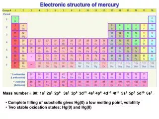
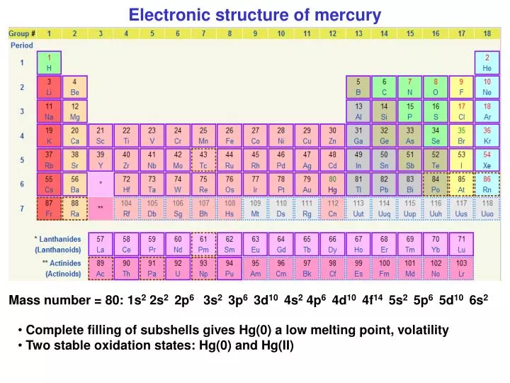
Electronic structure of mercury. Mass number = 80: 1s 2 2s 2 2p 6 3s 2 3p 6 3d 10 4s 2 4p 6 4d 10 4f 14 5s 2 5p 6 5d 10 6s 2. Complete filling of subshells gives Hg(0) a low melting point, volatility Two stable oxidation states: Hg(0) and Hg(II).

E N D
Electronic structure of mercury Mass number = 80: 1s2 2s2 2p6 3s2 3p6 3d10 4s2 4p6 4d10 4f14 5s2 5p6 5d10 6s2 • Complete filling of subshells gives Hg(0) a low melting point, volatility • Two stable oxidation states: Hg(0) and Hg(II)
Orbital energies vs. atomic number Energetic arrangement of orbitals is such that mercury (Z=80) has all its subshells filled
Biogeochemical cycle of mercury ANTHROPOGENIC PERTURBATION: fuel combustion mining WATER-SOLUBLE VOLATILE oxidation Hg(II) Hg(0) (months) volcanoes erosion ATMOSPHERE OCEAN/SOIL Hg(0) Hg(II) particulate Hg reduction biological uptake burial uplift SEDIMENTS
Global mercury deposition has roughly tripled since preindustrial times RISING MERCURY IN THE ENVIRONMENT Dietz et al. [2009]
HUMAN EXPOSURE TO MERCURY IS MAINLY FROM FISH CONSUMPTION Tuna is the #1 contributor Mercury biomagnification factor State fish consumption advisories EPA reference dose (RfD) is 0.1 μg kg-1 d-1 (about 2 fish meals per week)
Measuring Speciated Hg in the Atmosphere • GEM, RGM, and PBM drawn in through inlet • RGM collected on KCl denuder, HgP collected on particulate filter, and GEM passes through to be analyzed on 2537A. • RGM and HgP collected for 1-2hr. • HgP filter heated to 800°C and analyzed on 2537A as GEM. • RGM is thermally desorbed from KCl denuder at 500°C and analyzed on 2537A as GEM. Landis et al., 2002
Atmospheric transport of Hg(0) takes place on global scale Implies global-scale transport of anthropogenic emissions Anthropogenic Hg emission (2006) Mean Hg(0) concentration in surface air: circles = observed, background = GEOS-Chem model Transport around northern mid-latitudes: 1 month Hg(0) lifetime = 0.5-1 year Transport to southern hemisphere: 1 year Streets et al. [2009]; Soerensen et al. [2010]
LOCAL POLLUTION INFLUENCE FROM EMISSION OF Hg(II) High-temperature combustion emits both Hg(0) and Hg(II) 60% Hg(0) GLOBAL MERCURY POOL photoreduction 40% Hg(II) NEAR-FIELD WET DEPOSITION Hg(II) concentrations in surface air: circles = observed, background=model MERCURY DEPOSITION “HOT SPOT” Large variability of Hg(II) implies atmospheric lifetime of only days against deposition Thus mercury is BOTH a global and a local pollutant! Selin et al. [2007]
Atmospheric redox chemistry of mercury:what laboratory studies and kinetic theory tell us Older models X X OH, O3, Cl, Br Hg(II) Hg(0) X ? HO2(aq) • Oxidation of Hg(0) by OH or O3 is endothermic • Oxidation by Cl and Br may be important: • No viable mechanism identified for atmospheric reduction of Hg(II) Goodsite et al., 2004; Calvert and Lindberg, 2005; Hynes et al., UNEP 2008; Ariya et al., UNEP 2008
Atmospheric redox chemistry of mercury:what field observations tell us • Hg(0) lifetime against oxidation must be ~ months • Observed variability of Hg(0) • Oxidant must be photochemical • Observed late summer minimum of Hg(0) at northern mid-latitudes • Observed diurnal cycle of Hg(II) • Oxidant must be in gas phase and present in stratosphere • Hg(II) increase with altitude, Hg(0) depletion in stratosphere • Oxidation in marine boundary layer is by halogen radicals, likely Br • Observed diurnal cycle of Hg(II) • Oxidation can be very fast (hours-days) in niche environments during events • Boundary layer Hg(0) depletion in Arctic spring, Dead Sea from high Br Working hypothesis: Br atoms could provide the dominant global Hg(0) oxidant • If reduction happens at all it must be in the lower troposphere • Hg(II) increase with altitude, Hg(0) depletion in stratosphere • Hg(II)/Hg(0) emission ratios may be overestimated in current inventories • Lower-than-expected Hg(II)/Hg(0) observed in pollution plumes • Weaker-than-expected regional source signatures in wet deposition data
X ≡ Cl, Br, I organohalogen source radical cycling Halogen radical chemistry in troposphere: sink for ozone, NOx, VOCs, mercury sea salt source non-radical reservoir formation heterogeneous recycling
GOME-2 BrO columns Bromine chemistry in the atmosphere Inorganic bromine (Bry) O3 hv BrNO3 Br BrO Halons hv, NO OH HBr HOBr Stratospheric BrO: 2-10 ppt CH3Br Thule Stratosphere VSLS Tropopause (8-18 km) Troposphere TroposphericBrO: 0.5-2 ppt CHBr3 CH2Br2 OH, h Bry Satellite residual [Theys et al., 2011] debromination BrO column, 1013 cm-2 deposition Sea salt industry plankton
Mean vertical profiles of CHBr3 and CH2Br2 From NASA aircraft campaigns over Pacific in April-June Vertical profiles steeper for CHBr3 (mean lifetime 21 days) than for CH2Br(91 days), steeper in extratropics than in tropics Parrella et al. [2012]
Liang et al. [2010] stratospheric Bry model (upper boundary conditions) STRATOSPHERE 36 TROPOSPHERE Global tropospheric Bry budget in GEOS-Chem (Gg Br a-1) 56 Bry 3.2 ppt CH3Br Deposition 57 CH2Br2 lifetime 7 days 407 CHBr3 1420 (5-15) 7-9 ppt Marine biosphere Volcanoes Sea-salt debromination (50% of 1-10 µm particles) SURFACE Sea salt is the dominant global source but is released in marine boundary layer where lifetime against deposition is short; CHBr3 is major source in the free troposphere Parrella et al. [2012]
Tropospheric Bry cycling in GEOS-Chem Global annual mean concentrations in Gg Br (ppt), rates in Gg Br s-1 Gg Br (ppt) • Model includes HOBr+HBr in aq aerosols with = 0.2, ice with = 0.1 • Mean daytime BrO = 0.6 ppt; would be 0.3 ppt without HOBr+HBr reaction Parrella et al. [2012]
Zonal annual mean concentrations (ppt) in GEOS-Chem BrO • Bry is 2-4 ppt, highest over Southern Ocean (sea salt) • BrO increases with latitude(photochemical sink) • Br increases with altitude(BrO photolysis) Br Bry Parrella et al. [2012]
Comparison to seasonal satellite data for tropospheric BrO[Theys et al., 2011] (9:30 am) model model • TOMCAT has lower =0.02 for HOBr+HBrthan GEOS-Chem, large polar spring source from blowing snow • HOBr+HBr reaction critical for increasing BrO with latitude, winter/spring NH max in GEOS-Chem Parrella et al. [2012]
Effect of Br chemistry on tropospheric ozone Zonal mean ozone decreases (ppb) in GEOS-Chem • Two processes: catalytic ozone loss via HOBr, NOx loss via BrNO3 • Global OH also decreases by 4% due to decreases in ozone and NOx Parrella et al. [2012]
Bromine chemistry improves simulation of 19th century surface ozone • Standard models without bromine are too high, peak in winter-spring; bromine chemistry corrects these biases • Model BrO is similar in pre-industrial and present atmosphere (canceling effects) Parrella et al. [2012]
GEOS-Chem global mercury model • 3-D atmospheric simulation coupled to 2-D surface ocean and land reservoirs • Gas-phase Hg(0) oxidation by Br atoms • In-cloud Hg(II) photoreduction to enforce 7-month Hg lifetime against deposition Kinetics from Goodsite et al. [2004], Donohoue et al. [2005]; Balabanov et al. [2005] anthropogenic + geogenic primary emissions Hg(0) + Br ↔ Hg(I) → Hg(II) vegetation ocean mixed layer Hg(II) Hg(0) surface reservoirs ~ months Hg(II) Hg(0) soil stable reservoirs ~ decades natural + legacy boundary conditions
MERCURY WET DEPOSITION FLUXES,2004-2005 Circles: observations Background: GEOS-Chem model Model contribution from North American anthropogenic sources Model contribution from external sources Selin and Jacob [2008]
History of global anthropogenic Hg emissions Large past (legacy) contribution from N. American and European emissions; Asian dominance is a recent phenomenon Streets et al. , 2011
1977-2010 surface air trend of Hg(0) over the Atlantic Ocean • 1990-2010 data from ship cruises show a 50% decrease over North Atlantic, no significant trend over South Atlantic • Surface ocean Hg in North Atlantic also show a 50% decrease for 1990-2010, while subsurface Hg shows a 80% decrease [Mason et al., 2012] Cruises Mace Head Cruises Cape Point ocean mixed layer surface ocean 50-100 m subsurface ocean thermocline (~1000 m) Sørensenet al., submitted
GEOS-Chem simulation of Hg(0) 1990-2010 trends in surface air Forced by Streets emission trends Global 3-D atmospheric model coupled to 2-D surface ocean and land models, with subsurface ocean as boundary condition Forced by observed subsurface Atlantic trends ng m-3 a-1 • Simulation forced by 80% decrease in subsurface North Atlantic yields 50% decrease in surface air Hg(0) over 1990-2010, consistent with observations • Subsurface decrease must reflect a large decline in Hg inputs to the North Atlantic over 1970-2010. Sørensenet al., submitted
Decreasing Hg input to subsurface North Atlantic, 1970-20101. Atmospheric deposition explanation 1970 2000 Hg(0) Hg(0) Br Br marine boundary layer Hg(0) Hg(II) Hg(0) Hg(II) fast slow ocean mixed layer subsurface ocean (down to thermocline) • Hg deposition is thought to be driven by MBL oxidation of Hg(0) by Br atoms • MBL ozone ~doubled during 1970-2000; Br concentrations would have correspondingly decreased (Br/BrO photochemical equilibrium) O3 BrO Br h Sørensenet al., submitted
Decreasing Hg input to subsurface North Atlantic, 1970-20002. Disposal of Hg-containing commercial products 1970 2000 Disposed Hg-containing commercial products incineration Hg(II) Hg Hg wastewater, leaching N AMERICA, EUROPE Hg • Secondary wastewater treatment and phase-out of Hg from commercial products would have greatly decreased Hg input to the subsurface N Atlantic Sørensenet al., submitted
Disposal of Hg in commercial products:a missing component of the Hg biogeochemical cycle? Global production of commercial Hg peaked in 1970 Streets et al. [2011] and Hannah Horowitz (Harvard)
7-box model with 7 coupled ODEs dm/dt = s(t) – km where s is primary emission • Transfer rate constants k are specified from best knowledge Global biogeochemical model for mercury Primary emissions Model is initialized at natural steady state, and then forced with anthropogenic emissions for 2000 BC – present; % present-day enrichments are indicated Amos et al., submitted
7-box model with transfer rate constants Figure 1. Rate coefficients kij(a-1) driving our 7-compartment global biogeochemical box model for Hg. kij defines the first-order transferfrom reservoir i to reservoir j as Fij=kijmi, where Fij (Mg a-1) is the Hg flow from reservoir i to reservoir j and mi(Mg) is the mass of Hg in reservoir i.Values of kijare derived from best estimates of present-day flows and masses from the literature and are assumed to be constant in time. The red arrow represents the external forcing by primary emissions (geogenic or anthropogenic) from the deep mineral reservoir. Geogenic emissions are constant (90 Mg a-1) and anthropogenic emissions are time-dependent.
Time scale for dissipation of an atmospheric emission pulse Reservoir fraction Pulse gets transferred to subsurface ocean within a few years and stays there ~100 years, maintaining a legacy in the surface ocean Amos et al., submitted
Global source contributions to Hg in present-day surface ocean emissions pre-1850 natural • Human activity has increased 7x the Hg content of the surface ocean • Half of this human influence is from pre-1950 emissions • N America, Europe and Asia share similar responsibilities for anthropogenic Hg in present-day surface ocean ROW former USSR N America S America Europe Asia Amos et al., submitted
February 2009: Governing Council of UNEP agrees on need for global legally binding instrument on mercury • Goal is to complete negotiations by 2013 • In US; Clean Air Mercury Rule (CAMR) to reduce power plant emissions was struck down by courts in 2008; new effort is underway TOWARDS A GLOBAL MERCURY TREATY:Focus activity of United Nations Environmental Program (UNEP) • CHALLENGES: • How to regulate in the face of considerable uncertainty? • How to account for legacy mercury from past US and European emissions? • How to account for possible major effects of climate change?
Negotiations to be completed by 2013 Looking toward the future: UNEP global treaty for Hg Effect of zeroing global anthropogenic emissions by 2015 • Zeroing anthropogenic emissions would decrease ocean Hg by 30% by 2100, while keeping emissions constant would increase it by 40% • Elevated Hg in surface ocean will take centuries to fix; the only thing we can do in short term is prevent it from getting worse. Amos et al., submitted