Download
1 / 33
340 likes | 495 Views
Electronic Structure. Gordon Watson Chemistry Department, Kelso High School. Based on Presentations produced by David P. White University of North Carolina, Wilmington. Adv Higher Unit 1 Topic 1. Introduction.

E N D
Electronic Structure Gordon Watson Chemistry Department, Kelso High School Based on Presentations produced by David P. White University of North Carolina, Wilmington Adv Higher Unit 1 Topic 1 Unit 1.1 Electronic Structure
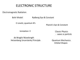
Introduction This topic describes the Electromagnetic Spectrum and how it can interact with atoms, Spectroscopy. Much information about Electronic Structure comes from spectroscopic evidence. Unit 1.1 Electronic Structure
The Wave Nature of Light • All waves have a characteristic wavelength,l,measured in metres (m) to nanometres (nm) • Thefrequency, n,of a wave is the number of waves which pass a point in one second measured in Hertz (Hz) or per seconds (s-1) • Thespeedof a wave,c, is given by its frequency multiplied by its wavelength: c = ν • For light,c = 3.00 x 10⁸ ms-1 • Another unit of ‘frequency’ used in spectroscopy is thewavenumber (1/λ), nu, measured in m-1or cm-1 Unit 1.1 Electronic Structure
Electromagnetic Radiation Unit 1.1 Electronic Structure
The Particle Nature of Light 1 • Planck: energy can only be absorbed • or released from atoms in • certain amounts calledquanta • To understandquantization, consider the notes produced by a violin (continuous) and a piano (quantized): • a violin can produce any note by placing the fingers at an appropriate spot on the fingerboard. • A piano can only produce certain notes corresponding to the keys on the keyboard. Unit 1.1 Electronic Structure
The Particle Nature of Light 2 Electromagnetic Radiation can also be thought of as a stream of very small particles known asphotons Electromagnetic Radiation exhibits wave-particledual properties. Theenergy (E) of aphoton(particle) is related to thefrequency(wave)of the radiation as follows: E = hν where h isPlanck’s constant ( 6.63 x 10⁻³⁴ J s ). Unit 1.1 Electronic Structure
Energy Calculations 1 • E = hν or E = h c / λ • Theenergycalculated would be in Joules (J) and would be a very small quantity. • Normally, we would calculate the energy transferred by the emissionor absorption ofone mole of photonsas follows: • E = Lhν or E = Lh c / λ • Where L is theAvogadro Constant, 6 .02 x 1023 and E would now be in J mol-1 or kJ mol-1. Unit 1.1 Electronic Structure
Energy Calculations 2 For example, a neon strip light emitted light with a wavelength of 640 nm. 640 nm = 640 x 10-9 m = 6.40 x 10⁻⁷ m. For eachphoton: E = h c / λ = 6.63 x 10-34 x 3.00 x 108 / 6.40 x 10-7 = 3.11 x 10⁻¹⁹ J For1 mole of photons: E = 3.11 x 10-19 x 6.02 x 1023 J = 1.87 x 10⁵ J mol-1 = 187 kJ mol-1 Unit 1.1 Electronic Structure
Emission Spectra 1 Atomic emissionspectraprovided significant contributions to the modern picture of atomic structure Radiation composed of only one wavelength is calledmonochromatic Radiation that spans a whole array of different wavelengths is calledcontinuous White light can be separated into a continuousspectrumof colors. Unit 1.1 Electronic Structure
Emission Spectra 2 Unit 1.1 Electronic Structure
Hydrogen Emission Spectrum Unit 1.1 Electronic Structure
Line Spectra The spectrum obtained when hydrogen atoms are excitedshows four lines: red, blue-green, blue and indigo Bohr deduced that the colours were due to the movement ofelectronsfrom a higher energy level back to the ‘ground state’. The significance of a Line Spectrum is that it suggests that electrons can only occupy certainfixed energy levels Unit 1.1 Electronic Structure
Bohr’s Model These fixed energy levels are what we have always called our electron shells A photon of light is emitted or absorbed when an electron changes from one energy level (shell) to another. Unit 1.1 Electronic Structure
Principal Quantum Number • Bohr described each shell by a number, • theprincipal quantum number, n • For the first shell,n = 1 • For the second shell,n = 2and so on. • After lots of math, Bohr showed that • where n is the principal quantum number (i.e.,n = 1, 2, 3,…), and RH is the Rydberg constant = 2.18 x 10⁻¹⁸ J. Unit 1.1 Electronic Structure
Hydrogen Spectra The lines detected in the visible spectrum were due to electrons returning to then=2level and are called theBalmer Series Another series of lines called theLyman Seriesare due to electrons returning to then=1level. The DE values are higher andthe lines appear in theultra-violetregion. Unit 1.1 Electronic Structure
Ionisation Energy 1 When we examine spectra we notice that each series of lines converge, i.e the gaps between the lines get smaller and smaller until the lines seem to merge. Frequency The line of greatest energy (lowest wavelength, highest frequency), represents an electron returning from the outer limit of an atom to the ground state ( n=1 in the case of Hydrogen). With slightly more energy the electron would have removed from the atom completely, i.e. the Ionisation Energy Unit 1.1 Electronic Structure
Ionisation Energy 2 For example, the wavelength of the line at the convergence Limit of the Lyman series in the Hydrogen spectrum is 91.2 nm. 91.2 nm = 91.2 x 10⁻⁹ m = 9.12 x 10⁻⁸ m. For eachphoton: E = h c / λ = 6.63 x 10-34 x 3.00 x 108 / 9.12 x 10-8 = 2.18 x 10⁻¹⁸ J For1 mole of photons: E = 2.18 x 10-18 x 6.02 x 1023 J = 1.31 x 10⁶ J mol-1 = 1,310 kJ mol-1 Data Book Value 1,311 kJ mol-1 Unit 1.1 Electronic Structure
Subshells - Orbitals High resolution spectra of more complex atoms reveal that lines are often split into triplets, quintuplets etc. This is evidence that Shells are further subdivided into Subshells These Subshells are called Orbitals Calculations using Quantum Mechanics have been able to determine the shapes of these Orbitals Unit 1.1 Electronic Structure
s-orbitals Quantum mechanics has shown that s orbitals are spherical in shape An orbital is a region in space where there is a greater than 90% probability of finding an electron. Unit 1.1 Electronic Structure
Orbitals and Quantum Numbers • Angular Quantum Number, l. This quantum number describes • the shape of an orbital. l = 0, 1, 2, and 3 (4 shapes) but we use letters for l (s, p, d and f). Usually we refer to the s, p, d and f-orbitals • Magnetic Quantum Number, ml. This quantum number describes the orientation of orbitals of the same shape. The magnetic quantum number has integral values between -l and +l. However, we use px , pyandpz instead. • There are 3 possible p -orbitals -1 0 +1 • There are 5 possible d-orbitals -2 -1 0 +1 +2 • There are 7 possible f-orbitals Unit 1.1 Electronic Structure
p-orbitals The shape of a p-orbital is dumb-bell, (l = 1). Each shell, from the second shell onwards, contains three of these p-orbitals, ( ml = -1 0 +1 ). We describe their orientation as ‘along the x-axis’, px‘along the y-axis’, py and ‘along the z-axis’, pz Unit 1.1 Electronic Structure
d-orbitals The shape of d-orbitals (l = 2) are more complicated. Each shell, from the third shell onwards, contains five of these d-orbitals, ( ml = -2 -1 0 +1 +2 ). We describe their orientation as ‘between the x-and y-axis’,dxy,‘between the x-and z-axis’,dxz,‘between the y-and z-axis’,dyz, ‘along the x- and y-axis’,dx2-y2and ‘along the z-axis’,dz2 Unit 1.1 Electronic Structure
f-orbitals The shape of f-orbitals (l = 3) are even more complicated. Each shell, from the fourth shell onwards, contains seven of these f-orbitals, ( ml = -3 -2 -1 0 +1 +2 +3 ). f-orbitals are not included in Advanced Higher so we will not have to consider their shapes or orientations, thank goodness! Unit 1.1 Electronic Structure
f-orbitals Couldn’t resist it ! Unit 1.1 Electronic Structure
Spin Quantum Number Each orbital can hold up to 2 electrons. In 1920 it was realised that an electron behaves as if it has a spin A fourth quantum number was needed. The spin quantum number, ms only has two values +1/2and - 1/2 Therefore, up tofour quantum numbers, n (shell), l (shape), ml (orientation) and ms (spin) are needed to uniquely describe every electron in an atom. Unit 1.1 Electronic Structure
Energy Diagram Orbitals can be ranked in terms of energy to yield anAufbau diagram As n increases, note that the spacing between energy levels becomes smaller. Sets, such as the 2p-orbitals, are of equal energy, they are degenerate Notice that the third and fourth shells overlap Unit 1.1 Electronic Structure
Electron Configurations 1 There are 3 rules which determine in which orbitals the electrons of an element are located. The Aufbau Principle states that electrons will fill orbitals starting with the orbital of lowest energy. For degenerate orbitals, electrons fill each orbital singly before any orbital gets a second electron (Hund’s Rule of Maximum Multiplicity). The Pauli Exclusion Principle states that the maximum number of electrons in any atomic orbital is two…….. and ….. if there are two electrons in an orbital they must have opposite spins (rather than parallel spins). Unit 1.1 Electronic Structure
Electron Configurations 2 Unit 1.1 Electronic Structure
Periodic Table Unit 1.1 Electronic Structure
Emission Spectroscopy 1 Li line: 2p 2s transition K line: 4p 4s transition Na line (589 nm): 3p 3s transition In emission spectroscopy, light of certain wavelengths is emitted as ‘excited’ electrons drop down from higher energy levels. The spectrum is examined to see the wavelengths emitted. Unit 1.1 Electronic Structure
Emission Spectroscopy 2 Each element provides a characteristic spectrum which can be used to identify the element. Analysing light from stars etc, tell us a lot about the elements present. The intensity of a particularly strong line in an element’s spectrum can be measured. The intensity of the light emitted is proportional to the quantity of the atoms/ions in the sample. Calibration samples can be prepared, intensities measured and unknown concentrations determined. Analytical tool. Unit 1.1 Electronic Structure
Absorption Spectroscopy In absorption spectroscopy, light of certain wavelengths is absorbed and electrons are promoted to higher energy levels. The spectrum is examined to see which wavelengths have been absorbed. The intensity of the light absorbed is proportional to the quantity of the atoms/ions in the sample. Calibration samples can be prepared, intensities measured and unknown concentrations determined (PPA) Unit 1.1 Electronic Structure
Electronic Structure of Atoms End of Topic 1 Unit 1.1 Electronic Structure