Download
1 / 20
230 likes | 370 Views
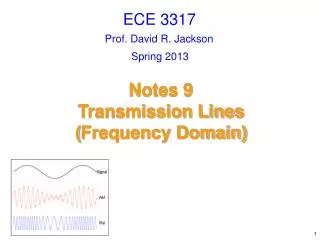
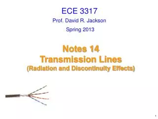
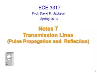
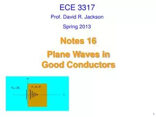
ECE 3317. Prof. David R. Jackson. Spring 2013. Notes 11 Transmission Lines ( Standing Wave Ratio (SWR) and Generalized Reflection Coefficient). Standing Wave Ratio. Z g. I( z ). +. Z 0. Sinusoidal source. V( z ). Z L. -. S. z = 0. z.

E N D
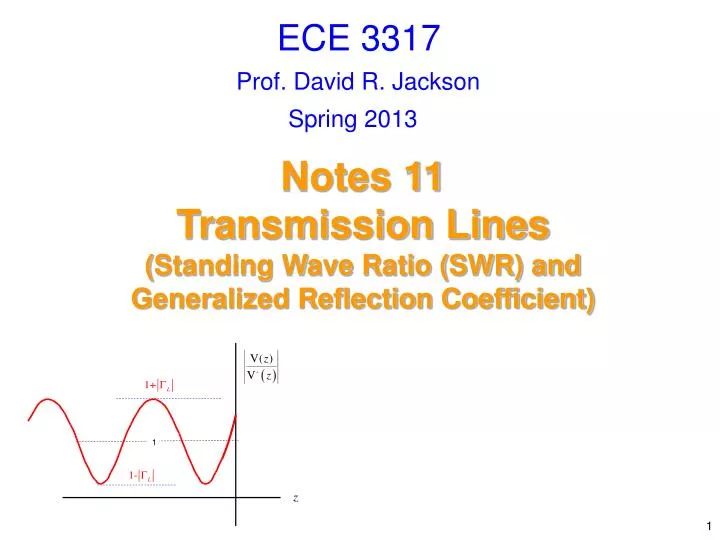
ECE 3317 Prof. David R. Jackson Spring 2013 Notes 11 Transmission Lines(Standing Wave Ratio (SWR) and Generalized Reflection Coefficient)
Standing Wave Ratio Zg I(z) + Z0 Sinusoidal source V(z) ZL - S z = 0 z Consider a lossless transmission line that is terminated with a load:
Standing Wave Ratio (cont.) Denote Then we have The magnitude is Maximum voltage: Maximum voltage:
Standing Wave Ratio (cont.) The voltage standing wave ratio is the ratio of Vmaxto Vmin . We then have For the current we have
Standing Wave Ratio (cont.) Hence we have The current standing wave ratio is thus Hence
Standing Wave Pattern Note: V+ is not in general the same as Vinc.
Crank Diagram where Note: 1 1 z Moving from load (angle change 2 z) Note: We go all the way around the crank diagram when z changes by / 2.
Standing Wave Ratio: Real Load Special case of a real load impedance Case a:
Standing Wave Ratio: Real Load (cont.) Hence Case b: Hence
Standing Wave Ratio: Real Load (cont.) Hence, for a real load impedance we have
Example (6.6, Shen and Kong) I(z) + Z0 V(z) ZL - z = 0 z Given: Find:
Example (6.6, Shen and Kong) (cont.) This problem has practical significance: often we are interested in figuring out what an unknown load is. Reverse problem: Given: What is the unknown load impedance? (Any multiple of 2 can be added.)
Example (6.6, Shen and Kong) (cont.) or The calculation yields
Generalized Reflection Coefficient z Zg S Z0 Sinusoidal source ZL z = 0 z0 Define the “generalized reflection coefficient” at a point z0on the line:
Generalized Reflection Coefficient Rearranging, we have Solve for L We can then write where
Generalized Reflection Coefficient (cont.) S where z z Zg Z0 Sinusoidal source ZL z = 0 z0 We identify (z0) as the reflection coefficient at the point z0. Hence
Generalized Reflection Coefficient (cont.) Define a normalized input impedance at point z0: We then have (This is the starting point for the Smith chart discussion.)
Example Z0 ZL Given: Calculate the reflection coefficient and the input impedance at z0 = -0.125 so so