Download
1 / 26
280 likes | 413 Views
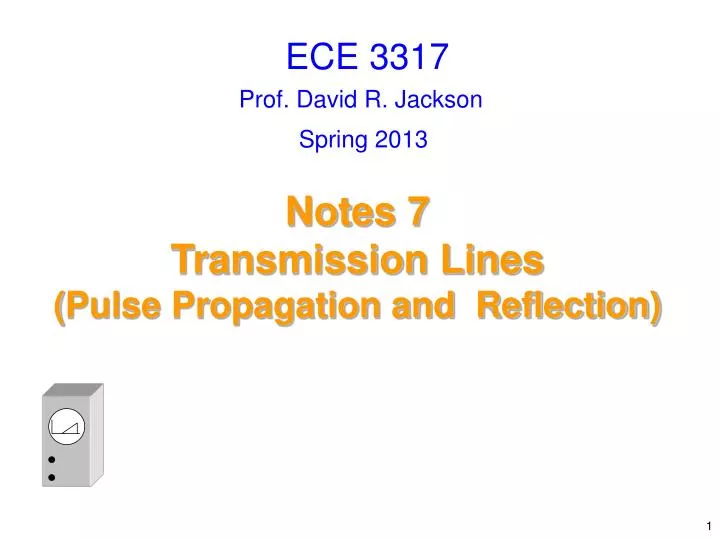
ECE 3317. Prof. David R. Jackson. Spring 2013. Notes 7 Transmission Lines ( Pulse Propagation and Reflection). Pulse on Transmission Line. z. +. -. z = 0. t. A voltage signal is applied at the input of the semi-infinite transmission line. Example:. Sawtooth wave.

E N D
ECE 3317 Prof. David R. Jackson Spring 2013 Notes 7 Transmission Lines(Pulse Propagation and Reflection)
Pulse on Transmission Line z + - z = 0 t A voltage signal is applied at the input of the semi-infinite transmission line. Example: Sawtooth wave
Pulse on Transmission Line (cont.) + - z = 0 Goal: determine the function f At z= 0: Hence
Pulse on Transmission Line (cont.) Pulse + - z = 0 At any position z, the pulse that is measured is the same as the input pulse, except that it is delayed by a time td =z / cd. Note that the shape of the pulse as a function of z is a scaled mirror image of the pulse shape as a function of t.
Pulse on Transmission Line (cont.) t Note the delay in the trace on this oscilloscope. z > 0 z = 0 z > 0 z = 0 t
Pulse on Transmission Line (cont.) The pulse is shown emerging from the source end of the line. A series of “snapshots” is shown. t = t1< t t = t2 = t t = t4 > t3 t = t3 > t2 t= 0 z = 0
Step Function Source t = 0 + V0 = 1 [V] - z = 0 Another example (battery and switch) 1.0 unit step function u(t) t
Step Function Source (cont.) t = t1 t = 0 t = t2 V0 cd t = 0 + V0 -
Step Function Source (cont.) V0 t = 0 + V0 - z = 0 Steady-state solution (t=)
Matched Load + Z0 RL - z = L z = 0 On line: (forward-traveling wave) At load: Hence, at z = L, the two relations are the same since RL = Z0. When the waveform hits the load end, it “sees” a continuation of the line. There is no reflection.
Absorption by Load This shows the sawtooth waveform propagating on a matched line. cd t = t5 t=0 t = t1 t = t6 t = t4 t = t2 t = t3 Z0 RL z = L z = 0 The pulse is shown emerging from the source end of the line, traveling down the line, and then being absorbed by the matched load.
Absorption by Load (cont.) Step function on matched line t = T t = t1 t = 0 t = t2 V0 t = 0 + RL V0 - z = L z = 0 Time to reach the load end: For t > T we have reached steady state: V(z,t) = V0 everywhere on the line.
Arbitrary Load Z0 RL z = L z = 0 On line: (known function) where Goal: solve for V-(z,t) At load:
Arbitrary Load (cont.) Z0 RL z = L z = 0 At load: Hence
Arbitrary Load (cont.) Define voltage of forward-traveling wave at the load voltage of backward-traveling wave at the load Then load reflection coefficient Define We then have
Arbitrary Load (cont.) Summary for load reflection load reflection coefficient Note: There is no reflection for a matched system (RL = Z0). Note:
Arbitrary Load (cont.) We now proceed to obtain (for arbitrary z) This is a known function: At the load: Use Hence we have Now let = t + z / cd: Hence The reflected wave is delayed from the load due to the distanceL - z.
Reflection Picture Reflected wave Incident wave Z0 RL z z = L z = 0 L - z • Notes: • The reflected wave is the mirror image of the incident wave, reduced in amplitude. • The reflected wave is delayed from the load after traveling a distance L-z. Substitute into argument Also, we have Hence
Reflection Picture Reflected wave Incident wave Z0 RL z z = L z = 0 L - z Time it takes to go from load to observation point z Time it takes to reach load
Reflections at Source End Re-reflected wave Reflected wave Rg Z0 RL z = L z = 0 After the reflected wave hits the source end, there may be another reflection. Here we allow the source to have a Thévenin resistance Rg. Note: In calculating the reflection from the source, we turn off the source voltage.
Complete Wave Picture Reflected wave Incident wave Rg Z0 RL z = L z = 0 Incident: Reflected: Re-reflected: Re-re-reflected: We'll stop here …but we could do more reflections.
Comments • The higher-order reflected waves get smaller, due to the reflection coefficients. • The bounce diagram (discussed in the next set of notes) gives us a convenient way or tracking all of the waves and determining the waveform observed at any point on the line, when the generator voltage is a step function or a pulse.
Example Reflected wave Incident wave Rg = 50 [] Z0 = 75 [], r = 2.1 RL= 100 [] z = L = 100 [m] z = 0 1.0 t
Example (cont.) Reflected wave Incident wave A AL Rg = 50 [] Z0 = 75 [], r = 2.1 RL= 100 [] z = L = 100 [m] z = 0 Incident: Reflected: Re-reflected: Re-re-reflected:
Example (cont.) Reflected wave Incident wave Rg = 50 [] Z0 = 75 [], r = 2.1 RL= 100 [] z = L = 100 [m] z = 0 Total voltage: L = 100 [m]