The Millimeter Regime

1. SMT Arizona 10m GBT West Virginia 100m IRAM 30m Spain The Millimeter Regime ASTE Chile 10m MOPRA Australia 22m CSO Hawaii 10.4m Onsala Sweden 20m JCMT Hawaii 15m Crystal Brogan (NRAO/NAASC) Nobeyama Japan 45m APEX Chile 12m LMT Mexico 50m ARO 12m Arizona

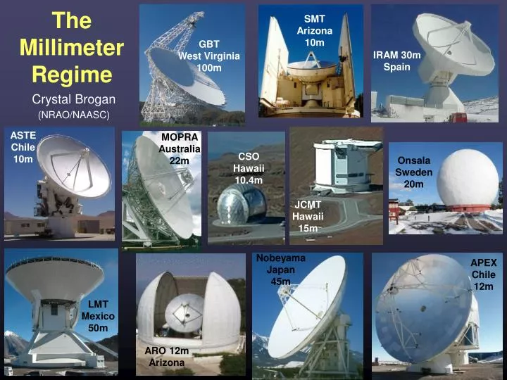
2. SMT Arizona 10m GBT West Virginia 100m IRAM 30m Spain • Outline • Effect of the Atmosphere at mm wavelengths • Effective System Temperature • Direct Method of mm calibration • Simplified formulation of Chopper Wheel method of mm calibration • More accurate approach • Efficiencies and different ways of reporting temperature • Why is mm so interesting? The Millimeter Regime ASTE Chile 10m MOPRA Australia 22m CSO Hawaii 10.4m Onsala Sweden 20m JCMT Hawaii 15m Crystal Brogan (NRAO/NAASC) Nobeyama Japan 45m APEX Chile 12m LMT Mexico 50m ARO 12m Arizona

3. Problems unique to the mm/sub-mm • Hardware • Noise diodes such as those used to calibrate the temperature scale at cm wavelengths are not available at mm to submm wavelengths Atmospheric opacity is significant for λ<1cm: raises Tsys and attenuates source Varies with frequency and altitude Changes as a function of time mostly due to H2O Causes refraction which leads to pointing errors Gain calibration must correct for these atmospheric effects • Antennas • Pointing accuracy measured as a fraction of the beam (PB ~ 1.22 l/D) is more difficult to achieve • Need more stringent requirements than at cm wavelengths for: surface accuracy and optical alignment

4. Column Density as a Function of Altitude Constituents of Atmospheric Opacity Due to the troposphere (lowest layer of atmosphere): h < 10 km Temperature decreases with altitude: clouds & convection can be significant Dry Constituents of the troposphere:, O2, O3, CO2, Ne, He, Ar, Kr, CH4, N2, H2 H2O: abundance is highly variable but is < 1% in mass, mostly in the form of water vapor “Hydrosols” (i.e. water droplets in the form of clouds and fog) also add a considerable contribution when present Stratosphere Troposphere

5. Opacity as a Function of PWV (PWV=Precipitable Water Vapor)

6. At 1.3cm most opacity comes from H2O vapor • At 7mm biggest contribution from dry constituents • At 3mm both components are significant • “hydrosols” i.e. water droplets (not shown) can also add significantly to the opacity total optical depth optical depth due to H2O vapor Optical Depth as a Function of Frequency optical depth due to dry air 43 GHz 7mm Q band 100 GHz 3mm MUSTANG 22 GHz 1.3cm K band

7. Effect of Atmosphere on Pointing • Since the refractive index of the atmosphere >1, an electromagnetic wave propagating through it will be bent which translates into a pointing offset • The index of refraction The amount of refraction is strongly dependent on the elevation • Pointing off-sets Δθ≈ 2.5x10-4 x tan(i) (radians) • @ elevation 45o typical offset~1’ • - GBT beam at 7mm is only 15”!

8. Consider the signal to noise ratio: • S / N = (Tsource e-t) / Tsys= Tsource / (Tsyset) • Tsys*=Tsyset≈Tatm(et -1) + Trxet • The system sensitivity (S/N) drops rapidly (exponentially) as opacity increases * Effective System Temperature (Tatm = temperature of the atmosphere ~ 270 K) Sensitivity: System noise temperature Receiver temperature Emission from atmosphere Before entering atmosphere the signalS= Tsource After attenuation by atmosphere the signal becomesS=Tsourcee- In addition to receiver noise, at millimeter wavelengths the atmosphere has a significant brightness temperature: Tsys≈ Trx + Tsky whereTsky =Tatm (1 – e-t) soTsys≈Trx +Tatm(1-e-t)

9. Atmospheric opacity, continued Typical optical depth for 230 GHz observing at the CSO: at zenitht225 = 0.15 = 3 mm PWV, at elevation = 30oÞt225 = 0.3 Tsys*(DSB) = et(Tatm(1-e-t) + Trec)= 1.35(77 + 75) ~ 200 K assuming Tatm = 300 K  Atmosphere adds considerably to Tsys and since the opacity can change rapidly, Tsys must be measured often Many MM/Submm receivers are double sideband, thus the effective Tsys for spectral lines (which are inherently single sideband) is doubled Tsys*(SSB) = 2 Tsys (DSB) ~ 400 K

10. Inverting this equation Where ηlaccounts for ohmic losses, rear spillover, and scattering and is < 1 Direct Method of MM Calibration TA’ is the antenna temperature of the source corrected as if it lay outside the atmosphere  at the observing frequency must be obtained by a tipping scan or some other means This is the method used at the GBT

11. Direct Calibration of the Atmosphere Tipping scan ηlaccounts for ohmic losses, rear spillover, and scattering and is < 1 With enough measurements at different elevation, ηl and  can be derived as long as reasonable numbers for the other parameters are known Trx: Receiver temp. from observatory Tatm ~ 260 K Tspill: Rear spillover temperature ~300 K Tcmb = 2.7 K

12. Atmosphere changes too rapidly to use average values http://www.gb.nrao.edu/~rmaddale/Weather/index.html For a forecast of current conditions Down side of the Direct Method • Tipping scans use considerable observing time ~10min each time • Probably not done often enough • Assume a homogeneous, plane-parallel atmosphere though the sky is lumpy • Done as a post-processing step so if something went wrong you’re out of luck

13. V Vhot + V rx Vcold +V rx T Tcold Thot -Treceiver Determining the Trx and the Temperature Scale In order to measure Trx, you need to make measurements of two calibrated ‘loads’: Tcold = 77 K liquid nitrogen load Thot = room temperature load Then and • Trx is not a constant, especially for mm/submm receivers which are more difficult to tune to ideal performance. • A significant improvement to the Tsys* measurement can be made if Trx is measured rather than assumed • Currently the SMA and soon ALMA will use a two temperature load system for all calibration and the temperature conversion factor is

14. We want to know the effective sensitivity, not how much is due to the receiver vs. how much is due to the sky. Therefore, we can use: Voff is the signal from the sky (but not on source) Vload is the signal from the hot load Chopper Measurement of Tsys* • So how do we measure Tsys* without constantly measuring Trx and the opacity?Tsys*≈Trxet + Tatm(et -1) • At shorter mm λ, Tsys*is usually obtained by occasionally placing an ambient temperature load (Thot) that has properties similar to a black body in front of the receiver. • As long as Tatm is similar to Thot, this method automatically compensates for rapid changes in mean atmospheric absorption IRAM 30m chopper Blue stuff is called eccosorb

15. Simplify by assuming that i.e., all our loads are at ambient temp. Then most everything cancels out and we are left with Recall from cm signal processing But instead of diode we have a BB load so and Simplified Load Calibration Theory Let Note that the load totally blocks the sky emission, which changes the calibration equations from cm result

16. So How Does This Help? Relating things back to measured quantities: To first order, ambient absorber (chopper wheel) calibration corrects for atmospheric attenuation! So all you have to do is alternate between Ton and Toff andoccasionally throw in a reading of Thot (i.e. a thermometer near your hot load) and a brief observation with Tload in the beam The poorer the weather, the more often you should observe Tload . This typically only takes a few seconds compared to ~10min for a tipping scan

17. 2. Let all temperatures be different: Millimeter-wave Calibration Formalism Corrections we must make: 1. At millimeter wavelengths, we are no longer in the R-J part of the Planck curve, so define a Rayleigh-Jeans equivalent radiation temperature of a Planck blackbody at temperature T. Once the function starts to curve, the assumption breaks down Linear part is in R-J limit

18. 3. Most millimeter wave receivers using SIS mixers have some response to the image sideband, even if they are nominally “single sideband”. (By comparison, HEMT amplifiers probably have negligible response to the image sideband.) • The atmosphere often has different opacity in the signal & image sidebands • Receiver gain must be known in the signal sideband Gs = signal sideband gain, Gi image sideband gain.

19. Commonly used TR* scale definition (recommended by Kutner and Ulich): • TR* includes all telescope losses except direct source coupling of the forward beam in d • The disadvantage is that fss is not a natural part of chopper wheel calibration and must be included as an extra factor • TA* is quoted most often. Either convention is OK, but know which one the observatory is using

20. Main Beam Brightness Temperature If the source angular extent is comparable to or smaller than the main beam, we can define a Main Beam Brightness Temperature as: fss the forward spillover and scattering can be measured from observations of the Moon, if moon = diffraction region M* -- corrected main beam efficiency – can measure from observations of planets which have mm Tb ~ few hundred K

21. Flux conversion factors (Jy/K) Conventional TA* definition

22. Why do we care about mm/submm? • mm/submm photons are the most abundant photons in the spectrum of most spiral galaxies – 40% of the Milky Way Galaxy • After the 3K cosmic background radiation, mm/submm photons carry most of the radiative energy in the Universe • Probe of cool gas and dust

23. Science at mm/submm wavelengths: dust emission In the Rayleigh-Jeans regime, hn « kT, Sn = 2kTn2tnW Wm-2 Hz-1 c2 and dust opacity, tnµ n2 so for optically-thin emission, flux density Snµ n4 Þemission is brighter at higher frequencies

24. Galactic star forming region NGC1333 Spitzer/IRAC image from c2d with yellow SCUBA 850 µm contours • Dust mass • Temperature • Star formation efficiency • Fragmentation • Clustering Jørgensen et al. 2006 and Kirk et al. 2006

25. Redshifting the steep FIR dust SED peak counteracts inverse square law dimming Increasing z redshifts peak SED peaks at ~100 GHz for z~10! Unique mm/submm access to highest z SED of Arp 220 at z=0.02 Andrew Blain

26. Science at mm/sub-mm wavelengths: molecular line emission Most of the dense ISM is H2, but H2 has no permanent dipole moment Þ use trace molecules • Plus: many more complex molecules (e.g. N2H+, CH3OH, CH3CN, etc) • Probe kinematics, density, temperature • Abundances, interstellar chemistry, etc… • For an optically-thin line Snµ n4; TBµ n2 (cf. dust)

27. List of Currently Known Interstellar Molecules H2 HD H3+ H2D+ CH CH+ C2 CH2 C2H *C3 CH3 C2H2 C3H(lin) c-C3H *CH4 C4 c-C3H2 H2CCC(lin) C4H *C5 *C2H4 C5H H2C4(lin) *HC4H CH3C2H C6H *HC6H H2C6 *C7H CH3C4H C8H *C6H6 OH CO CO+ H2O HCO HCO+ HOC+ C2O CO2 H3O+ HOCO+ H2CO C3O CH2CO HCOOH H2COH+ CH3OH CH2CHO CH2CHOH CH2CHCHO HC2CHO C5O CH3CHO c-C2H4O CH3OCHO CH2OHCHO CH3COOH CH3OCH3 CH3CH2OH CH3CH2CHO (CH3)2CO HOCH2CH2OH C2H5OCH3 NH CN N2 NH2 HCN HNC N2H+ NH3 HCNH+ H2CN HCCN C3N CH2CN CH2NH HC2CN HC2NC NH2CN C3NH CH3CN CH3NC HC3NH+ *HC4N C5N CH3NH2 CH2CHCN HC5N CH3C3N CH3CH2CN HC7N CH3C5N HC9N HC11N NO HNO N2O HNCO NH2CHO SH CS SO SO+ NS SiH *SiC SiN SiO SiS HCl *NaCl *AlCl *KCl HF *AlF *CP PN H2S C2S SO2 OCS HCS+ c-SiC2 *SiCN *SiNC *NaCN *MgCN *MgNC *AlNC H2CS HNCS C3S c-SiC3 *SiH4 *SiC4 CH3SH C5S FeO

28. The GBT PRIMOS Project:Searching for our Molecular Origins Many of these lines are currently unidentified! Hollis, Remijan, Jewell, Lovas

29. Detection of Acetamide (CH3CONH2): The Largest Molecule with a Peptide Bond (Hollis et al. 2006, ApJ, 643, L25) Detected in emission and absorption toward Sagittarius B2(N) using four A-species and four E-species rotational transitions. All transitions have energy levels less than 10 K. This molecule is interesting because it is one of only two known interstellar molecules containing a peptide bond. Thus it could provide a link to the polymerization of amino acids, an essential ingredient for life. GBT at 7mm

30. Comparison of GBT with mm Arrays All other things being equal, the effective collecting area (A) of a telescope is good measure of its sensitivity Telescope altitude diam. No. A nrange (feet) (m) dishes (m2) (GHz) GBT 2,650 100 1 1122* 80 - 115 SMA 13,600 6 8 230 220 - 690 CARMA 7,300 3.5/6/10 23 800 80 - 230 IRAM PdBI 8,000 15 6 1060 80 - 345 ALMA 16,400 12 50 5700 80 - 690 * Effective GBT collecting area at 3mm is ~10% compared to ~70% for others so GBT A/7 is listed

31. Summary • Effect of the Atmosphere at mm wavelengths • Attenuates source and adds noise • Effective System Temperature • Direct Method of mm calibration • Requires measurement of , used at GBT • Simplified formulation of Chopper Wheel method of mm calibration • Needed to replace diode method at shorter λs • More accurate approach • Planck, Different temperatures, Sidebands • Efficiencies and different ways of reporting temperature • Know what scale you are using • Why is mm so interesting? • Traces cool universe SMT Arizona 10m GBT West Virginia 100m IRAM 30m Spain The Millimeter Regime ASTE Chile 10m MOPRA Australia 22m CSO Hawaii 10.4m Onsala Sweden 20m JCMT Hawaii 15m Nobeyama Japan 45m APEX Chile 12m LMT Mexico 50m ARO 12m Arizona