Download
1 / 27
270 likes | 410 Views
Computing Price Trajectories in Combinatorial Auctions with Proxy Bidding. Jie Zhong Gangshu Cai Peter R. Wurman North Carolina State University. Overview. Problem Definition Intuition The Algorithm Conclusion. Proxy Bidding in Combinatorial Auctions.

E N D
Computing Price Trajectories in Combinatorial Auctionswith Proxy Bidding Jie ZhongGangshu CaiPeter R. WurmanNorth Carolina State University
Overview • Problem Definition • Intuition • The Algorithm • Conclusion
Proxy Bidding in Combinatorial Auctions • Bidders give a set of values to an agent • Agents place bids in an internal auction that solves the WDP and announces prices
Proxy Bidding Diagram Proxy Bids ValueStatement Auction ProxyBidder Final Prices,Winners Prices, Winners
Benefits • Speeds up auction • Simplifies the strategy space • Interactions with proxies may have several steps, allowing deferred computation of valuations
A Simple Iterative Combinatorial Auction • Bidders make offers on bundles of items • All bids are retained • Price bundles at highest bid • Inform current winners (not necessarily the highest bidders) • Non-winning bidders must beat price by d * this will not be a strategic analysis!
Proxy Bidding Rules • If the agent is not already winning something, it bids on the item that provides the most surplus • where is the price of bundle b. • Bid • If more than one b satisfies, then randomly select one.
The Proxy Auction Problem • PAP: Compute the final prices and allocation of a proxy auction given the bids • By Simulation • Agents bid • WDP and prices are computed • Repeat
Simulation is Undesirable Because… • Accuracy depends on bid increment • Slow: Solves multiple WDPs • Sensitive to magnitude of values • Sensitive to ordering of agents • Sensitive to tie-breaking rules • There is some regularity that we can take advantage of…
Some Observations • Periods of steady progress • Agents maintain a demand set • Spread bids among bundles in demand set • Punctuated by changes in behavior when • A new bundle is added to someone’s demand set • An agent drops out • An allocation becomes competitive and its members start passing
The Algorithm: Key Concepts • - Demand Set • The bundles that give an agent the maximal surplus at current prices. • - Attention • The proportion of time an agent spends bidding on a bundle in its demand set. • - Trajectory • The slope of the price of b,
Competitive Allocations • The set of competitive allocations (CAs) contains the solutions, f, with the maximal value, i.e., • Must account for bidders who are actively bidding and those who have stopped bidding • CAs have slopes: • CAs are winning with frequency
New Bundle Collisions • For Pb Pc • When the surplus that i gets from c is as good as from b, i will add c to its demand set • Special case: when the null bundle enters demand set, agent becomes inactive
Computing the Duration of an Interval • The interval is the amount of time until the next collision • Compute the earliest surplus collision(s) • Compute the earliest CA collision(s) • Select the min
At a Collision • When a collision occurs • Some bundles may leave demand sets • Some allocations may no longer be competitive • Thus, we know the potential demand sets and potential CAs, but not which will remain so in the next interval
Solving the Allocation of Attention, Demand Sets, & CAs s.t. Integer Variables: yi,b = 1 if b is in i’s demand set xf = 1 if f is competitive When b is in i’s demand set if c is also, their slopes are equal, Otherwise the slope of c is greater than b’s The sum of the frequencywith which CAs are selectedas winning is one. When f is competitive, if f^ is also, then their slopes are equal, otherwise the slope of f is greater than f^
Solving the Allocation of Attention, Demand Sets, & CAs s.t. If an agent is active, Ki = 1 Otherwise, Ki = 0 Each agent bids if it wasnot told it was winningi.e., whenever a CA to which it does not belong is selected Constraints to tie integer variables tocontinuous variables
The Algorithm: Main Loop • Solve the MILP to get • The demand set of each agent • The allocation of attention • The competitive allocations • Compute the duration of the interval,or terminate • Compute the prices at the end of the interval • Jump to end of interval and repeat
Anecdotal Comparison • Simulation: • With d = .005, took > 3000 iterations • Accuracy depends on d • Depends on tie-breaking rules, ordering of bidders • Price Trajectory Algorithm • 11 computations • Focused only on points at which the behavior changed • Exact computation of prices and allocation
Some Comments • Does not require complete value statements • The algorithm handles multiple value statements
Directions • Current implementation in AMPL • Working on a systematic comparison of performance • Improve computation time • Prove correspondence with simulation • Apply framework to other iterative combinatorial auctions