Table of Contents Chapter 5 (What-If Analysis for Linear Programming)

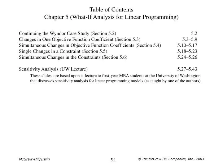
Continuing the Wyndor Case Study (Section 5.2) 5.2 Changes in One Objective Function Coefficient (Section 5.3) 5.3–5.9 Simultaneous Changes in Objective Function Coefficients (Section 5.4) 5.10–5.17 Single Changes in a Constraint (Section 5.5) 5.18–5.23 Simultaneous Changes in the Constraints (Section 5.6) 5.24–5.26 Sensitivity Analysis (UW Lecture) 5.27–5.43 These slides are based upon a lecture to first-year MBA students at the University of Washington that discusses sensitivity analysis for linear programming models (as taught by one of the authors). Table of ContentsChapter 5 (What-If Analysis for Linear Programming) © The McGraw-Hill Companies, Inc., 2003

Wyndor (Before What-If Analysis) © The McGraw-Hill Companies, Inc., 2003

Using the Spreadsheet to do Sensitivity Analysis The profit per door has been revised from $300 to $200.No change occurs in the optimal solution. © The McGraw-Hill Companies, Inc., 2003

Using the Spreadsheet to do Sensitivity Analysis The profit per door has been revised from $300 to $500.No change occurs in the optimal solution. © The McGraw-Hill Companies, Inc., 2003

Using the Spreadsheet to do Sensitivity Analysis The profit per door has been revised from $300 to $1,000.The optimal solution changes. © The McGraw-Hill Companies, Inc., 2003

Using Solver Table to do Sensitivity Analysis © The McGraw-Hill Companies, Inc., 2003

Using the Sensitivity Report to Find the Allowable Range © The McGraw-Hill Companies, Inc., 2003

Graphical Insight into the Allowable Range The two dashed lines that pass through the solid constraint boundary lines are the objective function lines when PD (the unit profit for doors) is at an endpoint of its allowable range, 0 ≤ PD≤ 750. © The McGraw-Hill Companies, Inc., 2003

Using the Spreadsheet to do Sensitivity Analysis The profit per door has been revised from $300 to $450.The profit per window has been revised from $500 to $400.No change occurs in the optimal solution. © The McGraw-Hill Companies, Inc., 2003

Using the Spreadsheet to do Sensitivity Analysis The profit per door has been revised from $300 to $600.The profit per window has been revised from $500 to $300.The optimal solution changes. © The McGraw-Hill Companies, Inc., 2003

The 100 Percent Rule The 100 Percent Rule for Simultaneous Changes in Objective Function Coefficients: If simultaneous changes are made in the coefficients of the objective function, calculate for each change the percentage of the allowable change (increase or decrease) for that coefficient to remain within its allowable range. If the sum of the percentage changes does not exceed 100 percent, the original optimal solution definitely will still be optimal. (If the sum does exceed 100 percent, then we cannot be sure.) © The McGraw-Hill Companies, Inc., 2003

Graphical Insight into 100 Percent Rule The estimates of the unit profits for doors and windows change to PD = $525 and PW = $350, which lies at the edge of what is allowed by the 100 percent rule. © The McGraw-Hill Companies, Inc., 2003

Graphical Insight into 100 Percent Rule When the estimates of the unit profits for doors and windows change to PD = $150 and PW = $250 (half their original values), the graphical method shows that the optimal solution still is (D, W) = (2, 6) even though the 100 percent rule says that the optimal solution might change. © The McGraw-Hill Companies, Inc., 2003

Using the Spreadsheet to do Sensitivity Analysis The hours available in plant 2 have been increased from 12 to 13.The total profit increases by $150 per week. © The McGraw-Hill Companies, Inc., 2003

Using the Spreadsheet to do Sensitivity Analysis The hours available in plant 2 have been further increased from 13 to 18.The total profit increases by $750 per week ($150 per hour added in plant 2). © The McGraw-Hill Companies, Inc., 2003

Using the Spreadsheet to do Sensitivity Analysis The hours available in plant 2 have been further increased from 18 to 20.The total profit does not increase any further. © The McGraw-Hill Companies, Inc., 2003

Using the Sensitivity Report © The McGraw-Hill Companies, Inc., 2003

Graphical Interpretation of the Allowable Range © The McGraw-Hill Companies, Inc., 2003

Using the Spreadsheet to do Sensitivity Analysis One available hour in plant 3 has been shifted to plant 2.The total profit increases by $50 per week. © The McGraw-Hill Companies, Inc., 2003

The 100 Percent Rule The 100 Percent Rule for Simultaneous Changes in Right-Hand Sides: The shadow prices remain valid for predicting the effect of simultaneously changing the right-hand sides of some of the functional constraints as long as the changes are not too large. To check whether the changes are small enough, calculate for each change the percentage of the allowable change (decrease or increase) for that right-hand side to remain within its allowable range. If the sum of the percentage changes does not exceed 100 percent, the shadow prices definitely will still be valid. (If the sum does exceed 100 percent, then we cannot be sure.) © The McGraw-Hill Companies, Inc., 2003

A Production Problem Weekly supply of raw materials: 8 Small Bricks 6 Large Bricks Products: Table Profit = $20 / Table Chair Profit = $15 / Chair © The McGraw-Hill Companies, Inc., 2003

Sensitivity Analysis Questions • With the given weekly supply of raw materials and profit data, how many tables and chairs should be produced? What is the total weekly profit? • What if one more large brick were available. How much would you be willing to pay for it? • What if an additional two large bricks were available (to make a total of 9). How much would you be willing to pay for these two additional bricks? • What if the profit per table were now $25. (Assume now there are only 6 large bricks again.) How many tables and chairs should now be produced? • What if the profit per table were now $35. How many tables and chairs should now be produced? © The McGraw-Hill Companies, Inc., 2003

Graphical Solution (Original Problem) Maximize Profit = ($20)T + ($15)Csubject to 2T + C ≤ 6 large bricks 2T + 2C ≤ 8 small bricksandT ≥ 0, C ≥ 0. © The McGraw-Hill Companies, Inc., 2003

7 Large Bricks Maximize Profit = ($20)T + ($15)Csubject to2T + C ≤ 7 large bricks 2T + 2C ≤ 8 small bricksandT ≥ 0, C ≥ 0. © The McGraw-Hill Companies, Inc., 2003

9 Large Bricks Maximize Profit = ($20)T + ($15)Csubject to 2T + C ≤ 9 large bricks 2T + 2C ≤ 8 small bricksandT ≥ 0, C ≥ 0. © The McGraw-Hill Companies, Inc., 2003

$25 Profit per Table Maximize Profit = ($25)T + ($15)Csubject to 2T + C ≤ 6 large bricks 2T + 2C ≤ 8 small bricksandT ≥ 0, C ≥ 0. © The McGraw-Hill Companies, Inc., 2003

$35 Profit per Table Maximize Profit = ($35)T + ($15)Csubject to 2T + C ≤ 6 large bricks 2T + 2C ≤ 8 small bricksandT ≥ 0, C ≥ 0. © The McGraw-Hill Companies, Inc., 2003

Generating the Sensitivity Report After solving with Solver, choose “Sensitivity” under reports: © The McGraw-Hill Companies, Inc., 2003

The Sensitivity Report Allowable range(Solution stays the same) The solution Usage of the resource(Left-hand-side of constraint) Allowable range(Shadow price is valid) Increase in objective function value per unit increase in right-hand-side (RHS)∆Z = (shadow price)(∆RHS) © The McGraw-Hill Companies, Inc., 2003

100% Rule for Simultaneous Changesin the Objective Coefficients For simultaneous changes in the objective coefficients, if the sum of the percentage changes does not exceed 100%, the original solution will still be optimal. (If it does exceed 100%, we cannot be sure—it may or may not change.) Examples: (Does solution stay the same?) Profit per Table = $24 & Profit per Chair = $13Profit per Table = $25 & Profit per Chair = $12Profit per Table = $28 & Profit per Chair = $18 © The McGraw-Hill Companies, Inc., 2003

100% Rule for Simultaneous Changesin the Right-Hand-Sides For simultaneous changes in the right-hand-sides, if the sum of the percentage changes does not exceed 100%, the shadow prices will still be valid. (If it does exceed 100%, we cannot be sure—they may or may not be valid.) Examples: (Are the shadow prices valid? If so, what’s the new total profit?) (+1 Large Brick) & (+2 Small Bricks)(+1 Large Brick) & (–1 Small Brick) © The McGraw-Hill Companies, Inc., 2003

Summary of Sensitivity Report for Changes in the Objective Function Coefficients • Final Value • The value of the decision variables (changing cells) in the optimal solution. • Reduced Cost • Increase in the objective function value per unit increase in the value of a zero-valued variable (for small increases)—may be interpreted as the shadow price for the nonnegativity constraint. • Objective Coefficient • The current value of the objective coefficient. • Allowable Increase/Decrease • Defines the range of the coefficients in the objective function for which the current solution (value of the decision variables or changing cells in the optimal solution) will not change. © The McGraw-Hill Companies, Inc., 2003

Summary of Sensitivity Report for Changes in the Right-Hand-Sides • Final Value • The usage of the resource (or level of benefit achieved) in the optimal solution—the left-hand side of the constraint. • Shadow Price • The change in the value of the objective function per unit increase in the right-hand-side of the constraint (RHS): ∆Z = (Shadow Price)(∆RHS)(Note: only valid if change is within the allowable range—see below.) • Constraint R.H. Side • The current value of the right-hand-side of the constraint. • Allowable Increase/Decrease • Defines the range of values for the RHS for which the shadow price is valid and hence for which the new objective function value can be calculated. (NOT the range for which the current solution will not change.) © The McGraw-Hill Companies, Inc., 2003

Table of Contents Chapter 5 (What-If Analysis for Linear Programming)