Download
1 / 61
620 likes | 783 Views
Electromagnetic Wave Propagation Prof. V.K. Tripathi Department of Physics IIT Delhi October 26, 2007. Core Issue. How does a signal Propagate from a transmitter to a receiver?. Transmitter. Receiver. (1). (2). Signal.

E N D
Electromagnetic Wave Propagation Prof. V.K. Tripathi Department of Physics IIT Delhi October 26, 2007
Core Issue How does a signal Propagate from a transmitter to a receiver? Transmitter Receiver
(1) (2) Signal On the path of a propagating signal if we measure the electric field, we find a rapidly oscillating electric field E. In the simplest form : where A is amplitude ω is frequency in rad s-1 and The real part of RHS is implied in Eq.(2) If we measure the magnetic field, we get
Signal Propagation Z z = 0 t = 0 z = z t = t
where, and
A plane of constant phase i.e., kz = constant; Signal propagates along z, i.e. perpendicular to the wavefront ⋀ A plane perpendicular to z ⋀ k z z = 0 wavefront ⋀ Wavefront
Q M ^ r n : direction of wave propagation y Wavefront θ ⋀ n x O Oblique Propagation If vp is the phase velocity,
⋀ ⋀
^ ^ Example Obtain the amplitude, frequency, wavelength, phase velocity and equation of the wavefront. Solution Compare this equation with
^ ^ ^ ^ ^ Wavefront : = constant
Under what conditions is a solution of Maxwell’s Equations? • What is ω Vs k relation (dispersion relation)? • B = ? Major Issues
Faraday’s law of Electromagnetic Induction conduction current density displacement current density Maxwell’s Equations
^ ^ ^ (We will take = 0)
(when G is constant) ^ ^ ^ ^ ^ ^ An Important Identity
i.e. = j k when operates over a quantity that varies as over a quantity that varies as Hence. Similarly,
If LHS of an equation has phase variation as , RHS must also have it. • If , then from B must vary as • Similarly must vary in the same way. • Hence replace in Maxwell’s equations, reducing them to algebraic equations and Another Important Observation
Algebraic form of Maxwells’ Equations • jk . D = • j k . B = 0(i.e. B is perpendicularto k) • j k E = jω B = jω H • j k H = J jω D = E jω E
Since j k H = J jω D = E jω E effective relative permittivity Effective Relative Permittivity
(1) (2) Taking ( k ) of the first equation and using the second, (3) (4) Relevant Set when = 0
k E eff ≠ 0 for ( k . ) of this equation gives This gives the dispersion relation
E B k Main Result for a plane EM Wave
E ^ ⋀ x k ⋀ ^ ⋀ z B y EM Wave in Vacuum A wave propagating along z may be taken as
In a Dielectric Dispersion: When rdepends on ω, refractive index depends on ω and the medium is called dispersive, e.g. glass.
^ ^ ^ ^ ^ ^ Example: An em wave propagating in a dielectric has Obtain , vp, r Comparing this expression with
Conductivity e: electronic charge m: electron effective mass ω: frequency of the electric field (of the wave) : collision frequency (~1012 s-1) n0: free electron density (~1022 cm-3)
kis real for k is imaginary for we depict k = j amplitude Special cases: ω >> • Phase has no dependence • on z • Amplitude falls off with z
Skin depth for ω >> No energy propagation ωplasmaedge ω
Skin depth increases as ωdecreases Special case ω<<
Shorter frequencies penetrate deeper into a conductor. This fact is employed in Magneto-Telluric technique of underground exploration. • E/H ratio at the earth surface for • ω ~ 110 Hz gives effective permittivity on the earth at different depths. Applications Generator-detector eff Earth Burried ore
ω ωp kr For ω < ωpno propagation Forω > ωp
Poynting Vector S : energy flow per unit area per unit time S = E H = Re E ReH Energy Flow Using the identity
time average = 0 Sav is called intensity
Example The amplitude of a laser in free space is 10 V m-1. Estimate its intensity. Solution:
ωp = ωcos θi Height from ground (km) θ 600 EARTH 300 IONOSPHERE 10 107 104 Short Wave Communication Plasma density n0 increases with height upto 300 km, then it falls off.
An obliquely incident em wave into the ionosphere moves away from vertical (as the medium becomes optically rarer). From Snell’s law, horizontal component of kremains unchanged. Short waves in ionosphere
At the turning point, θ = /2 i.e. ωp = ω cos θi Wave suffers reflection from a height where
z r θ y l x Intuitive generalization with retarded time: A(r, t) must depend on current in the wire at time t’ = t – r/c Antenna Antenna is an exposed portion of wire through which an ac current of frequency ω flows. If it were a dc current:
⋀ Radiation term Induction term ⋀
^ ^ ^ ^ ^
⋀ z dl r θ Radiated intensity ~ ω2 ~ sin2 ( is the angle between antenna length and r ) Saveis maximum for
Save θ Radiation Pattern xy plane xz plane locus of the tip of Save as varies locus of the tip of Save as varies
x Free space (0) z x = 0 0 Conductor (eff ) Surface Wave A wave that propagates along the interface of a conductor and free space (or dielectric). Its amplitude falls off away from the interface. Boundary condition at x = 0, i.e., the tangential (Ez) component of electric field be continuous, demands that the phase variation in both media be same (except dependence on x) We take phase variation of E as
^ ^ In vacuum we may write: Comparing it with
Inside the conductor : Boundary conditions at x = 0 EzI= EzIIandExI = eff ExII A1z = A2z
ω kz Dispersion relation Field amplitude falls off with | x | The decline is more rapid inside conductor.
Antenna Earth Medium Wave Communication Earth conductivity: ~ 1mho m-1, Attenuation length ~1000 km at 3 MHz. At high frequency (short waves), attenuation is sever hence SW communication is via ionospheric reflection. MW signals can be detected at hundreds of meters of height. Surface waves bend whenever there are bends or curvature on the surface of the earth.