Download
1 / 33
370 likes | 949 Views
Principles of Biostatistics Chapter 17 Correlation. 宇传华 http://statdtedm.6to23.com 网上免费统计资源(八). Terminology. scatter plot 散点图 correlation 相关 linear correlation 直线 相关 correlation coefficient 相关系数

E N D
Principles of Biostatistics Chapter 17 Correlation 宇传华http://statdtedm.6to23.com 网上免费统计资源(八)
Terminology scatter plot散点图 correlation 相关 linear correlation 直线相关 correlation coefficient 相关系数 Pearson’s correlation coefficient Pearson相关系数 Spearman’s rank correlation coefficient Spearman等级相关系数
CONTENTS §17.1 The Two-Way Scatter Plot §17.2 Pearson’s Correlation Coefficient: r §17.3 Spearman’s Correlation Coefficient: rs §17.4 Further Application
Correlation (coefficient) The correlation between two random variables, X and Y, is a measure (指标)of the degree of linear association between the two variables. The population correlation, denoted by (Greek letter, Symbol字体,读音rou) The sample correlation, denoted byr(Latin letter or English letter), (r)can take on any value from -1 to 1. (r) indicates a perfect negative linear relationship indicates a perfect positive linear relationship indicates no linear relationship The absolute value of indicates the strength(强度) of the relationship. -1< <0 indicates a negative linear relationship 0< <1 indicates a positive linear relationship The sign of indicates the Direction(方向)of the relationship.
One statistical technique often employed to measure such an association is known as correlation analysis Before we conduct correlation analysis, we should always created a two-way scatter plot (scatter diagram). X variable------horizontal axis Y variable------vertical axis; each point on the graph represents a combination value (Xi,Yi). Through scatter plot,we can often determine whether a linear relationship exists between X and Y.
§17.1 The Two-Way Scatter Plot 表 凝血酶浓度(X)与凝血时间(Y)间的关系
Perfect positive Strong positive Positive correlation r = 1 correlation r = 0.99 correlation r = 0.80 Strong negative No correlation Non-linear correlation correlation r = -0.98 r = 0.00
The important of a scatter plot In the next chapter (simple linear regression), we also need a scatter plot to find if the relationship between X and Y is a linear relationship, if the relationship between X and Y is a positive linear relationship. So, before the analysis of correlation and regression, we should usually make a scatter plot
§17.2 Pearson’s correlation coefficient (r) Synonyms: product moment (积矩) correlation coefficient simple linear(简单线性) correlation coefficient Definition: r-------A statistical index to describe the intensity (strength) and the direction of association between two variables (X,Y). r is a dimensionless number(无量纲数);it has no units of measurement -1≤r ≤ 1
X,Y: random variables following normal distribution (Bivariate Normal Distribution). both Xi and Yi are measured from the same subject ith
Sx Sy Sx2 Sy2 Sxy
2) Calculation of r lXX=0.404,lYY=22.933,lXY=-2.82 X,Y : stronger negative relationship
Inference about correlation coefficient r ---------- hypothesis test • Establish testinghypothesis , determining significant level α H0 : =0 no linear association between X and Y H1 : ≠0 linear association between X and Y exists =0.05 two-sided probability of type I error
2) Calculating statistic =n-2 For the above example =15-2=13 From t distribution table (Table A4,Appendix), the critical value is t0.05/2(13)=2.160 < |t|=8.874, P<0.05, Correlation coefficient is statistically significant at α=0.05. concentration of thrombin and clotting time are negatively related.
§17.3 Spearman’s Rank Correlation Coefficient: rs Spearman等级相关系数 rank 可翻译为: 秩,等级 Spearman‘s rank correlation (a method of nonparametric test )is applied if two variables are distributed far fromnormal. • i.e. the normality requirement is not satisfied
The steps of hypothesis test Rank ordering according to its magnitude of values for each of the two variables (Xi,Yi) (Xri,Yri) Calculating the Spearman’s rank correlation coefficient based on the ranks
For tie (equal) ranks, mean rank is used instead. Six ‘–’s, mean=(1+2+3+4+5+6)/6=3.5
Because there are some tie ranks in Y we can not use the formula latter.
Explanation of Spearman’s rank correlation coefficient: rs (1) -1≤rs≤1 and similar meaning as r does (2) Difference between rsand r. rs≠ r Calculated by original values of data Calculated by ranks
Statistical inference about rs 1) Setting uphypothesis, determining significant level H0:s=0 H1:s0 =0.05 2) Calculating test statistic 3) Conclusion: No association between platelet(血小板) and bleeding(出血).
Y Y Y X X X Notices in application 1. r=0 does not mean no correlation (might be non-linear correlation) H0:r =0 H0:r =0 H0:r =0
Notices in application • When levels of either variable X or Y are artificially selected, it is not suitable to make Pearson’s correlation analysis ( but we can do spearman’s rank correlation analysis). Pearson’s correlation analysis requires that both X and Y follows normal distribution.
Notices in application 3. Outliers can affect correlation coefficient heavily.
Notices in application 4. Correlation cause-effect association(因果联系), Correlation intrinsic association(固有联系). 5. The difference between statistical significance (P value) intensity of correlation (absolute value of r) : There are statisticalsignificance of correlation coefficient ------ the probability of r from the =0is small (P value is small). Intensity of correlation ----the absolute value of r
§17.4 Further Application SAS Codes for textbook’s Table 17.1 and Table 17.2 89 124 95 10 87 6 91 33 98 16 73 32 47 145 76 87 90 9 ; PROCCORRPEARSONSPEARMAN; VAR X Y; RUN; DATA EXP17_12; INPUT X Y; CARDS; 77 118 69 65 32 184 85 8 94 43 99 12 89 55 13 208 95 7 95 9 54 9
The CORR Procedure 2 Variables: X Y Simple Statistics Variable N Mean Std Dev Median Minimum Maximum X 20 77.40000 23.65409 88.00000 13.00000 99.00000 Y 20 59.00000 63.86581 32.50000 6.00000 208.00000 Pearson Correlation Coefficients, N = 20 Prob > |r| under H0: Rho=0 X Y X 1.00000 -0.79107 <.0001 Y -0.79107 1.00000 <.0001 Spearman Correlation Coefficients, N = 20 Prob > |r| under H0: Rho=0 X Y X 1.00000 -0.54319 0.0133 Y -0.54319 1.00000 0.0133
SAS Codes for textbook’s Table 17.3 and Table 17.4 37 800 35 500 96 60 55 100 90 10 96 5 99 5 99 8 95 120 ; PROCCORRPEARSONSPEARMAN; VAR X Y; RUN; DATA EXP17_34; INPUT X Y; CARDS; 5 600 100 3 98 67 84 170 100 6 99 15 70 120 50 170 26 300 6 830 100 10
The CORR Procedure 2 Variables: X Y Simple Statistics Variable N Mean Std Dev Median Minimum Maximum X 20 72.00000 33.79193 92.50000 5.00000 100.00000 Y 20 194.95000 268.92211 83.50000 3.00000 830.00000 Pearson Correlation Coefficients, N = 20 Prob > |r| under H0: Rho=0 X Y X 1.00000 -0.87681 <.0001 Y -0.87681 1.00000 <.0001 Spearman Correlation Coefficients, N = 20 Prob > |r| under H0: Rho=0 X Y X 1.00000 -0.88969 <.0001 Y -0.88969 1.00000 <.0001
SUMMARY • Simple linear correlation coefficient: r • Condition: Both X and Y variables • follow the normal distribution. • Spearman’s rank correlation coefficient: rs • It does not require that X or Y follows the normal distribution.
Assignment Review Exercises 5. (pp. 412)