Download
1 / 83
840 likes | 1.04k Views
The Radiobiology Behind Dose Fractionation Bill McBride Dept. Radiation Oncology David Geffen School Medicine UCLA, Los Angeles, Ca. wmcbride@mednet.ucla.edu. Objectives. To understand the mathematical bases behind survival curves Know the linear quadratic model formulation

E N D
The Radiobiology Behind Dose Fractionation Bill McBrideDept. Radiation OncologyDavid Geffen School MedicineUCLA, Los Angeles, Ca.wmcbride@mednet.ucla.edu
Objectives • To understand the mathematical bases behind survival curves • Know the linear quadratic model formulation • Understand how the isoeffect curves for fractionated radiation vary with tissue and how to use the LQ model to change dose with dose per fraction • Understand the 4Rs of radiobiology as they relate to clinical fractionated regimens and the sources of heterogeneity that impact the concept of equal effect per fraction • Know the major clinical trials on altered fractionation and their outcome • Recognize the importance of dose heterogeneity in modern treatment planning
Relevance of Radiobiology to Clinical Fractionation Protocols Conventional treatment: Tumors are generally irradiated with 2Gy dose per fraction delivered daily to a more or less homogeneous field over a 6 week time period to a specified total dose The purpose of convenntional dose fractionation is to increase dose to the tumor while PRESERVING NORMAL TISSUE FUNCTION • Deviating from conventional fractionation protocol impacts outcome • How do you know what dose to give; for example if you want to change dose per fraction or time? Radiobiological modeling provide the guidelines. It uses • Radiobiological principles derived from preclinical data • Radiobiological parameters derived from clinical altered fractionation protocols • hyperfractionation, accelerated fractionation, some hypofractionation schedules The number of non-homogeneous treatment plans (IMRT) and extreme hypofractionated treatments are increasing. Do existing models cope?
In theory, knowing relevant radiobiological parameters one day may predict the response for • Dose given in a single or a small number of fractions • SBRT, SRS, SRT, HDR or LDR brachytherapy, protons, cyberknife, gammaknife • Non-uniform dose distributions optimized by IMRT • e.g. dose “painting” of radioresistant tumor subvolumes • Combination therapies with chemo- or biological agents • Different RT options when tailored by molecular and imaging theragnostics • If you know the molecular profile and tumor phenotype, can you predict the best delivery method? • Biologically optimized treatment planning
The First Radiation Dosimeter prompted the use of dose fractionation
Modeling Radiation Responses P survival (when x = 0) 100 targets 100 hits m=1 e-1=0.368 100 targets 200 hits m=2 e-2=0.137 100 targets 300 hits m=3 e-3=0.05 Assumes that ionizing ‘hits’ are random events in space Which are fitted by a Poisson Distribution P of x = e-m.mx/x! where m = mean # hits, x is a hit N.B. Lethal hits in DNA are not really randomly distributed, e.g. condensed chromatin is more sensitive, but it is a reasonable approximation
This Gives a Survival Curve Based on a Model where one hit will eliminate a single target • When there is single lethal hit per target S.F.= e-1 = 0.37 • This is the mean lethal dose D0 • D10 = 2.3 xD0 • In general, S.F. = e-D/D0 or LnS.F. = -D/D0 or S.F. = e-aD , i.e. D0 = 1/a Where a is the slope of the curve and D0 the reciprocal of the slope 1.0 0.1 0.01 0.001 0.37 S.F. D0 How many logs of cells would be killed by 23 Gy if D0 = 1 Gy? D10 DOSE Gy
Puck and Marcus, J.E.M.103, 563, 1956First in vitro mammalian survival curve Eukaryotic Survival Curves are Exponential, but have a ‘Shoulder’ Two component model single lethal hits n 1.0 0.1 0.01 0.001 Accumulation of sub-lethal damage dose
Two Component Model • Two Component Model • (or single target, single hit + multi-target (n), single hit) • S.F.=e-D/1D0[1-(1-e-D/nD0)n] single lethal hits n 1.0 0.1 0.01 0.001 1D0 = reciprocal initial slope nD0 = reciprocal final slope S.F. Extrapolation Number Single hit Accumulated damage Accumulation of sublethal damage DOSE Gy
Mean Inactivation Dose (Do) • Virus D0 approx. = 1500 Gy • E. Coli D0 approx. = 100 Gy • Mammalian bone marrow cells D0 = 1 Gy • Generally, for mammalian cells D0 = 1-1.5 Gy Why the differences?
In general, history has shown repeatedly that single high doses of radiation do not allow a therapeutic differential between tumor and critical normal tissues. Dose fractionation does. SBRT/SRS often aims at TISSUE ABLATION
“Double Trouble” Does this Matter? Prescribed Dose: 25 fractions of 2Gy = 50Gy Hot spot: 110% Physical dose: 55Gy Biological dose: 60.5Gy
Linear Quadratic Model 1.0 0.1 0.01 0.001 • Cell kill is the result of single lethal hits plus accumulated damage from 2 independent sublethal events • The generalized formula is E = aD + bD2 • For a fractionated regimen E= nd(a + bd) = D (a + bd) Where d = dose per fraction and D = total dose • a/b is dose at which death due to single lethal lesions = death due to accumulation of sublethal lesions i.e.aD = bD2 and D = a/b in Gy aD S.F. = e-aD Single lethal hits bD2 S.F. S.F. = e-(aD+bD2) Single lethal hits plus accumulated damage a/ in Gy DOSE Gy
Over 90% of radiation oncologists use the LQ model: • it is simple and has a microdosimetric underpinning • a/b is large (> 6 Gy) when survival curve is almost exponential and small (1-4 Gy) when shoulder is wide • the a/b value quantifies the sensitivity of a tissue/tumor to fractionated radiation. • But: • Both a and b vary with the cell cycle. At high doses, S phase and hypoxic cells become more important. • The a/b ratio varies depending upon whether a cell is quiescent or proliferative • The LQ model best describes data in the range of 1 - 6Gy and should not be used outside this range
The Linear Quadratic Formulation • Does not work well at high dose/fx • Assumes equal effect per fraction
HT29 cells N.B. Survival curves may deviate from L.Q. at low and high dose!!!! • Certain cell lines, and tissues, are hypersensitive at low doses of 0.05-0.2Gy. • The survival curve then plateaus over 0.05-1Gy • Not seen for all cell lines or tissues, but has been reported in skin, kidney and lung • At high dose, the model probably does not fit data well because D2 dominates the equation Lambin et al. Int J Radiat Biol 63:639 1993
1 limiting slope/ low dose rate S.F. .1 5 fractions 3 fractions Single dose .01 0 0 4 8 12 16 20 24 Dose (Gy) • Multi-fraction survival curves can be considered linear if sublethal damage is repaired between fractions • they have an extrapolation number (n) = 1.0 • The resultant slope is the effective D0 • eD0 is often 2.5 - 5.0Gy and eD10 5.8 - 11.5Gy • S.F. = e-D/eD0 • If S.F. after 2Gy = 0.5, eD0 = 2.9Gy; eD10 = 6.7Gy and 30 fractions of 2 Gy (60Gy) would reduce survival by (0.5)30 = almost 9 logs (or 60/6.7) • If a 1cm tumor had 109 clonogenic cells, there would be an average of 1 clonogen per tumor and cure rate would be about 37%
Thames et al Int J Radiat Oncol Biol Phys 8: 219, 1982. • The slope of an isoeffect curve changes with size of dose per fraction depending on tissue type • Acute responding tissues have flatter curves than do late responding tissues • measures the sensitivity of tumor or tissue to fractionation i.e. it predicts how total dose for a given effect will change when you change the size of dose fraction Reciprocal total dose for an isoeffect Slope = Douglas and Fowler Rad Res 66:401, 1976 Showed and easy way to arrive at an ratio Intercept = Dose per fraction
1 .1 .01 Response to Fractionation Varies With Tissue 1 Acute Responding Tissues a/b = 10Gy Fractionated Late Effects S.F. S.F. Fractionated Acute Effects .1 Late Responding Tissues - a/b = 2Gy Single Dose Late Effects a/b = 2Gy Single Dose Acute Effects a/b = 10Gy a/b is high (>6Gy) when survival curve is almost exponential and low (1-4Gy) when shoulder is wide .01 0 0 4 8 12 16 20 0 0 4 8 12 16 Dose (Gy) Dose (Gy) Fractionation spares late responding tissues
80 70 60 50 40 30 20 20 30 40 50 60 70 80 =3Gy; 1.5Gy/fx =30Gy; 1.5Gy/fx 2.0Gy/fx =30Gy; 4Gy/fx D new =3Gy; 4Gy/fx D old Note how badly late responding tissues respond to increased dose/fraction
Sensitivity of Tissue to Dose Fractionation can be estimated by the ratio
In fact, for some tumors e.g. prostate, breast, melanoma, soft tissue sarcoma, and liposarcoma a/ ratios may be moderately low Prostate Brenner and Hall IJROBP 43:1095, 1999 comparing implants with EBRT a/ ratio is 1.5 Gy [0.8, 2.2] Lukka JCO 23: 6132, 2005 Phase III NCIC 66Gy 33F in 45days vs 52.5Gy 20F in 28 days Compatible with a/ ratio of 1.12Gy (-3.3-5.6) Breast Owen, J.R., et al. Lancet Oncol, 7: 467-471, 2006 and Dewar et al JCO, ASCO Proceedings Part I. Vol 25, No. 18S: LBA518, 2007. UK START Trial 50Gy in 25Fx c.w. 39Gy in 13Fx; or 41.6Gy in 13Fx [or 40Gy in 15Fx (3 wks)] Breast Cancer a/ = 4.0Gy (1.0-7.8) Breast appearance a/ = 3.6Gy; induration a/ = 3.1Gy What are a/ ratios for human cancers? If fractionation sensitivity of a cancer is similar to dose-limiting healthy tissues, it may be possible to give fewer, larger fractions without compromising effectiveness or safety
What total dose (D) to give if the dose/fx (d) is changed NewOld Dnew (dnew + ) = Dold (dold +) So, for late responding tissue, what total dose in 1.5Gy fractions is equivalent to 66Gy in 2Gy fractions? Dnew (1.5+2) = 66 (2 + 2) Dnew = 75.4Gy NB: Small differences in for late responding tissues can make a big difference in estimated D!
Biologically Effective Dose (BED) S.F. = e-E = e-(aD+bD2) E = nd(a + bd) E/a = nd(1+d/a/b) Biologically Effective Dose Relative Effectiveness Total dose 35 x 2Gy = B.E.D.of 84Gy10 and 117Gy3 NOTE: 3 x 15Gy = B.E.D.of 113Gy10 and 270Gy3 Normalized total dose2Gy = BED/RE = BED/1.2 for of 10Gy = BED/1.67 for of 3Gy Equivalent to 162 Gy in 2Gy Fx -unrealistic! (Fowler et al IJROBP 60: 1241, 2004)
700R 1500R Repopulation Redistribution Repair 4Rs OF DOSE FRACTIONATION • Assessed by varying the time between 2 or more doses of radiation
4Rs OF DOSE FRACTIONATION These are radiobiological mechanisms that impact the response to a fractionated course of radiation therapy • Repair of sublethal damage • spares late responding normal tissue preferentially • Redistribution of cells in the cell cycle • increases acute and tumor damage, no effect on late responding normal tissue • Repopulation • spares acute responding normal tissue, no effect on late effects, • danger of tumor repopulation • Reoxygenation • increases tumor damage, no effect in normal tissues
Repair • “Repair” between fractions should be complete - N.B. we are dealing with tissue recovery rather than DNA repair • Correction for incomplete repair is possible (Thames) • In general, time between fractions for most tissues should be >6 hours • Some tissues, such as CNS, recover slowly making b.i.d. treatment inadvisable • Bentzen - RadiotherOncol 53, 219, 1999 • CHART analysis HNC showed that late morbidity was less than would be expected assuming complete recovery between fractions • Is the T1/2 for recovery for late responding normal tissues 2.5-4.5hrs?
Regeneration in Normal Tissues • The lag time to regeneration varies with the tissue • In acute responding tissues, • Regeneration has a considerable sparing effect • In human mucosa, regeneration starts 10-12 days into a 2Gy Fx protocol and increases tissue tolerance by at least 1Gy/dy • Prolonging treatment time has a sparing effect • As treatment time is reduced, acute responding tissues become dose-limiting • In late responding tissues, • Prolonging overall treatment time beyond 6wks has little effect, but prolonging time to retreatment may increase tissue tolerance
Repopulation in Tumor Tissue Rat rhabdosarcoma Human SCC head and neck T2 T3 70 55 40 local control Total Dose (2 Gy equiv.) no local control Treatment Duration 4 weeks to start of accelerated repopulation. Thereafter T1/2 of 4 days = loss of 0.6Gy per day Withers, H.R., Taylor, J.M.G., and Maciejewski, B. Acta Oncologica 27:131, 1988 Hermens and Barendsen, EJC 5:173, 1969 Treatment breaks are often “bad”
Altered FractionationorHow to optimally distribute dose over time
Players • Total dose (D) • Dose per fraction (d) • Interval between fractions (t) • Overall treatment time (T) • Tumor type • Acute reacting normal tissues • Late reacting normal tissues
Tumor control Late responding tissue complications Complication-free cure Accelerated Fractionation Hyperfractionation TCP or NTC TCP or NTC Dose
S.F hypoxic oxic Dose Other Sources of Heterogeneity • Biological Dose • Cell cycle • Hypoxia/reoxygenation • Clonogenic “stem cells” (G.F.) • Number • Intrinsic radiosensitivity • Proliferative potential • Differentiation status • Physical Dose • Need to know more about the importance of dose-volume constraints Phillips, J Natl Cancer Inst 98:1777, 2006
Heterogeneity within and between between tumors in dose-response characteristics, often resulting in large error bars for values • In spite of this, the outcome of clinical studies of altered fractionation generally fit the models, within the constraints of the clinical doses used
Definitions • Conventional fractionation • Daily doses (d) of 1.8 to 2 Gy • Dose per week of 9 to 10 Gy • Total dose (D) of 40 to 70 Gy • Hyperfractionation • The number of fractions (N) is increased • T is kept the same • Dose per fraction (d) less than 1.8 Gy • Two fractions per day (t) Rationale:Spares late responding tissues
Definitions • Accelerated fractionation • Shorter overall treatment time • Dose per fraction of 1.8 to 2 Gy • More than 10 Gy per week Rationale:Overcome accelerated tumor repopulation • Hypofractionation • Dose per fraction (d) higher than 2.2 Gy • Reduced total number of fractions (N) Rationale: Tumor has low a/b ratio and there is no therapeutic advantage to be gained with respect to late complications
Very acceleratedwith reduction of dose 54 Gy - 36 fx - 12 days Moderately accelerated 72 Gy - 42 fx - 6 wks Hyperfractionated 81.6 Gy - 68 fx - 7 wks Conventional 70 Gy - 35 fx - 7 wks
HyperfractionatedBarcelona (586), Brazil (112), RTOG 90-03 (1113), EORTC 22791 (356), Toronto (331) Very acceleratedCHART (918), Vancouver (82), TROG 91-01 (350),GORTEC 94-02 (268) Moderately acceleratedRTOG 90-03 (1113), DAHANCA (1485), EORTC 22851 (512) CAIR (100), Warsaw (395) OtherEORTC 22811 (348), RTOG 79-13 (210) 7623 patients in 18 randomized phase III trials !! HNSCC only will be discussed
80.5 Gy - 70 fx - 7 wks control: 70 Gy - 35-40 fx - 7-8 wks EORTC hyperfractionation trial in oropharynx cancer (N = 356) Oropharyngeal Ca T2-3, N0-1 Horiot 1992 SURVIVAL p = 0.08 LOCAL CONTROL p = 0.02 Years Years
Very Accelerated: CHART (N = 918) Dische 1997 54 Gy - 36 fx - 12 days control: 66 Gy - 33 fx - 6.5 wks Loco-regional control Survival conventionalCHART conventionalCHART Favourable outcome with CHART: well differentiated tumors larynx carcinomas
P = 0.04 P = 0.003 Moderate/severe subcutaneousfibrosis and oedema Mucosal ulceration anddeep necrosis P = 0.04 P = 0.009 Laryngeal oedema Moderate/severe dysphagia CHART: Morbidity Dische 1997 54 Gy - 36 fx - 12 days control: 66 Gy - 33 fx - 6.5 wks
Moderately Accelerated Overgaard 2000 DAHANCA 6: only glottic, (N = 694)DAHANCA 7: all other sites, + nimorazole (N = 791) 66-68 Gy - 33-34 fx - 6 wks control: 66-68 Gy - 33-34 fx - 7 wks Actuarial 5-year rates Local controlDAHANCA 6 DAHANCA 7 Nodal controlDAHANCA 6 + 7 . Disease-specific survival DAHANCA 6 + 7 Overall survival Late effects (edema, fibrosis) 5 fx/wk 6 fx/wk 73% 81% p=0.04 56% 68% p=0.009 87% 89% n.s. 65% 72% p=0.04 n.s. n.s.
Moderately Accelerated OVERALL SURVIVAL CAIR Probability CONTROL log-rank p=0.00001 Follow-up (months) CAIR: 7-day-continuous accelerated irradiation (N = 100) Skladowski 2000 66-72 Gy - 33-36 fx - 5 wks control: 70-72 Gy - 35-36 fx - 7 wks68.4-72 Gy - 38-40 fx - 5.5 wks control: 66.6-72 Gy - 37-40 fx - 7.5-8 wks
Hyperfractionated 81.6 Gy - 68 fx - 7 wks RTOG 90-03, Phase III comparison of fractionation schedules in Stage III and IV SCC of oral cavity, oropharynx, larynx, hypopharynx (N = 1113) Fu 2000 Conventional 70 Gy - 35 fx - 7 wks Accelerated with split 67.2 Gy - 42 fx - 6 weeks (including 2-week split) Accelerated with Concomitant boost 72 Gy - 42 fx - 6 wks
RTOG 90-03,loco-regional control Fu 2000
RTOG 90-03, survival Fu 2000
RTOG 90-03, adverse effects Fu 2000 Acute Maximum toxicity Conventional Hyperfract Concom Acc +per patient boost split Grade 1 15% 4% 4% 7%Grade 2 57% 39% 36% 41%Grade 3 35% 54% 58% 49%Grade 4 0% 1% 1% 2% Late Maximum toxicity Conventional Hyperfract Concom Acc +per patient boost split Grade 1 11% 8% 7% 16%Grade 2 50% 56% 44% 50%Grade 3 19% 19% 29% 20%Grade 4 8% 9% 8% 7%Grade 5 1% 0% 1% 1%
Toxicity of RT in HNSCC Acute effects in accelerated or hyperfractionated RT Author Regimen Grade 3-4 mucositis Cont Exp Horiot (n=356) HF 49% 67% Horiot (n=512) Acc fx + split 50% 67% Dische (n=918) CHART 43% 73% Fu (n=536) Acc fx(CB) 25% 46% Fu (n=542) Acc fx + split 25% 41% Fu (n=507) HF 25% 42% Skladowski (n=99) Acc fx 26% 56%
Randomized trials 1970-1998 (no postop RT) 15 trials included (6515 patients) Survival benefit: 3.4% (36% 39% at 5 years, p = 0.003)Loco-regional control benefit: 7% (46.5% 53% at 5 years, p < 0.0001) Bourhis, Lancet 2006 Altered fractionation in head and neck cancer: meta-analysis
Conclusions for HNSCC • Hyperfractionation increases TCP and protects late responding tissues • Accelerated treatment increase TCP but also increases acute toxicity • What should be considered standard for patients treated with radiation only? • Hyperfractionated radiotherapy • Concomitant boost accelerated radiotherapy • Fractions of 1.8 Gy once daily when given alone, cannot be considered as an acceptable standard of care • TCP curves for SSC are frustratingly shallow … selection of tumors?