Download
1 / 35
370 likes | 593 Views
Genome Assembly: a brief introduction. Slides courtesy of Mihai Pop, Art Delcher, and Steven Salzberg. Shotgun DNA Sequencing (Technology). DNA target sample. SHEAR. SIZE SELECT. e.g., 10Kbp ± 8% std.dev. End Reads (Mates). 550bp. LIGATE & CLONE. Primer. SEQUENCE. Vector.

E N D
Genome Assembly: a brief introduction Slides courtesy of Mihai Pop, Art Delcher, and Steven Salzberg
Shotgun DNA Sequencing (Technology) DNA target sample SHEAR SIZE SELECT e.g., 10Kbp ± 8% std.dev. End Reads (Mates) 550bp LIGATE & CLONE Primer SEQUENCE Vector
Whole Genome Shotgun Sequencing + single highly automated process + only three library constructions – assembly is much more difficult • Collect 10x sequence in a 1-to-1 ratio of two types of read pairs: ~ 35million reads for Human. Short Long 10Kbp 2Kbp • Collect another 20X in clone coverage of 50Kbp end sequence pairs: ~ 1.2million pairs for Human. • Early simulations showed that if repeats were considered black boxes, one could still cover 99.7% of the genome unambiguously. BAC 3’ BAC 5’
Celera’s Sequencing Factory(circa 2001) • 300 ABI 3700 DNA Sequencers • 50 Production Staff • 20,000 sq. ft. of wet lab • 20,000 sq. ft. of sequencing space • 800 tons of A/C (160,000 cfm) • $1 million / year for electrical service • $10 million / month for reagents
Human Data (April 2000) • Collected 27.27 Million reads = 5.11X coverage • 21.04 Million are paired (77%) = 10.52 Million pairs • 2Kbp 5.045M 98.6% true * <6% std.dev. • 10Kbp 4.401M 98.6% true * <8% std.dev. • 50Kbp 1.071M 90.0% true * <15% std.dev. * validated against finished Chrom. 21 sequence • The clones cover the genome 38.7X times • Data is from 5 individuals (roughly 3X, 4 others at .5X)
Pairs Give Order & Orientation Contig Assembly without pairs results in contigs whose order and orientation are not known. Consensus (15- 30Kbp) Reads ? 2-pair Pairs, especially groups of corroborating ones, link the contigs into scaffolds where the size of gaps is well characterized. Mean & Std.Dev. is known Scaffold
Anatomy of a WGS Assembly STS Chromosome STS-mapped Scaffolds Contig Gap (mean & std. dev. Known) Read pair (mates) Consensus Reads (of several haplotypes) SNPs External “Reads”
Assembly gaps Physical gaps Sequencing gaps sequencing gap - we know the order and orientation of the contigs and have at least one clone spanning the gap physical gap - no information known about the adjacent contigs, nor about the DNA spanning the gap
Typical contig coverage Imagine raindrops on a sidewalk
Lander-Waterman statistics L = read length T = minimum detectable overlap G = genome size N = number of reads c = coverage (NL / G) σ = 1 – T/L E(#islands) = Ne-cσ E(island size) = L((ecσ – 1) / c + 1 – σ) contig = island with 2 or more reads
Example Genome size: 1 Mbp Read Length: 600 Detectable overlap: 40
Experimental data Caveat: numbers based on artificially chopping up the genome of Wolbachia pipientis dMel
Assembly paradigms • Overlap-layout-consensus • greedy (TIGR Assembler, phrap, CAP3...) • graph-based (Celera Assembler, Arachne) • Eulerian path (especially useful for short read sequencing)
TIGR Assembler/phrap Greedy • Build a rough map of fragment overlaps • Pick the largest scoring overlap • Merge the two fragments • Repeat until no more merges can be done
Overlap-layout-consensus Main entity: read Relationship between reads: overlap 1 4 7 2 5 8 3 6 9 2 3 4 5 6 7 8 9 1 ACCTGA ACCTGA AGCTGA ACCAGA 1 2 3 2 3 1 1 2 3 3 1 1 2 3 1 3 2 2
Paths through graphs and assembly • Hamiltonian circuit: visit each node (city) exactly once, returning to the start Genome
Overlap between two sequences overlap (19 bases) overhang (6 bases) …AGCCTAGACCTACAGGATGCGCGGACACGTAGCCAGGAC CAGTACTTGGATGCGCTGACACGTAGCTTATCCGGT… overhang % identity = 18/19 % = 94.7% • overlap - region of similarity between regions • overhang - un-aligned ends of the sequences • The assembler screens merges based on: • length of overlap • % identity in overlap region • maximum overhang size.
All pairs alignment • Needed by the assembler • Try all pairs – must consider ~ n2 pairs • Smarter solution: only n x coverage (e.g. 8) pairs are possible • Build a table of k-mers contained in sequences (single pass through the genome) • Generate the pairs from k-mer table (single pass through k-mer table) k-mer
Assembly Pipeline A B implies TRUE A B OR A B REPEAT-INDUCED Trim & Screen Find all overlaps 40bp allowing 6% mismatch. Overlapper Unitiger Scaffolder Repeat Rez I, II
Assembly Pipeline Trim & Screen Compute all overlap consistent sub-assemblies: Unitigs (Uniquely Assembled Contig) Overlapper Unitiger Scaffolder Repeat Rez I, II
OVERLAP GRAPH A A B B B A B A A B A B Edge Types: Regular Dovetail Prefix Dovetail Suffix Dovetail E.G.: Edges are annotated with deltas of overlaps
The Unitig Reduction A C A B C B 1. Remove “Transitively Inferrable” Overlaps:
The Unitig Reduction A 412 352 A B B 45 2. Collapse “Unique Connector” Overlaps:
Identifying Unique DNA Stretches Repetitive DNA unitig Unique DNA unitig Arrival Intervals Discriminator Statistic is log-odds ratio of probability unitig is unique DNA versus 2-copy DNA. +10 -10 0 Dist. For Unique Dist. For Repetitive Definitely Repetitive Don’t Know Definitely Unique
Assembly Pipeline Mated reads Scaffold U-unitigs with confirmed pairs Trim & Screen Overlapper Unitiger Scaffolder Repeat Rez I, II
Assembly Pipeline Trim & Screen Fill repeat gaps with doubly anchored positive unitigs Overlapper Unitig>0 Unitiger Scaffolder Repeat Rez I, II
Handling repeats • Repeat detection • pre-assembly: find fragments that belong to repeats • statistically (most existing assemblers) • repeat database (RepeatMasker) • during assembly: detect "tangles" indicative of repeats (Pevzner, Tang, Waterman 2001) • post-assembly: find repetitive regions and potential mis-assemblies. • Reputer, RepeatMasker • "unhappy" mate-pairs (too close, too far, mis-oriented) • Repeat resolution • find DNA fragments belonging to the repeat • determine correct tiling across the repeat
Statistical repeat detection Significant deviations from average coverage flagged as repeats. - frequent k-mers are ignored - “arrival” rate of reads in contigs compared with theoretical value (e.g., 800 bp reads & 8x coverage - reads "arrive" every 100 bp) Problem 1: assumption of uniform distribution of fragments - leads to false positives non-random libraries poor clonability regions Problem 2: repeats with low copy number are missed - leads to false negatives
Mis-assembled repeats excision collapsed tandem rearrangement