Download
1 / 47
480 likes | 594 Views
Explore efficient data-parallel primitives and algorithms for GPU computing, including scan, sort, and more. Learn about exclusive & inclusive scans, segmented scan challenges & implementations, and platform specifics for NVIDIA CUDA and G80.

E N D
Scan Primitives for GPU Computing Shubho Sengupta, Mark Harris*, Yao Zhang, John Owens University of California Davis, *NVIDIA Corporation
Motivation • Raw compute power and bandwidth of GPUs increasing rapidly • Programmable unified shader cores • Ability to program outside the graphics framework • However lack of efficient data-parallel primitives and algorithms
4 3 2 1 7 8 0 1 5 4 1 2 7 6 3 4 Motivation • Current efficient algorithms either have streaming access • 1:1 relationship between input and output element
4 3 8 1 7 7 0 4 5 4 1 7 9 6 3 3 Motivation • Or have small “neighborhood” access • N:1 relationship between input and output element where N is a small constant
0 Null 3 0 7 0 4 1 0 3 3 7 4 1 3 Motivation • However interesting problems require more general access patterns • Changing one element affects everybody • Stream Compaction
T F F T F F T F F F F F F T T T Motivation • Split • Needed for Sort
Motivation • Common scenarios in parallel computing • Variable output per thread • Threads want to perform a split – radix sort, building trees • “What came before/after me?” • “Where do I start writing my data?” • Scan answers this question
System Overview Libraries and Abstractions for data parallel programming Algorithms Sort, Sparse matrix operations,… Higher Level Primitives Enumerate, Distribute,… Low Level Primitives Scan and variants
3 0 3 1 4 3 11 4 7 0 11 11 4 11 15 1 15 16 22 16 6 22 3 25 Input Exclusive Inclusive Scan • Each element is a sum of all the elements to the left of it (Exclusive) • Each element is a sum of all the elements to the left of it and itself (Inclusive)
Scan – the past • First proposed in APL (1962) • Used as a data parallel primitive in the Connection Machine (1990) • Guy Blelloch used scan as a primitive for various parallel algorithms (1990)
Scan – the present • First GPU implementation by Daniel Horn (2004), O(n logn) • Subsequent GPU implementations by • Hensley (2005) O(n logn), Sengupta (2006) O(n), Greß (2006) O(n) 2D • NVIDIA CUDA implementation by Mark Harris (2007), O(n), space efficient
Scan – the implementation • O(n) algorithm – same work complexity as the serial version • Space efficient – needs O(n) storage • Has two stages – reduce and down-sweep
3 1 7 0 4 1 6 3 3 4 7 7 4 5 6 9 3 4 7 11 4 5 6 14 3 4 7 11 4 5 6 25 Scan - Reduce • log n steps • Work halves each step • O(n) work • In place, space efficient
3 4 7 11 4 5 6 25 3 4 7 11 4 5 6 0 3 4 7 0 4 5 6 11 3 0 7 4 4 11 6 16 0 3 4 11 11 15 16 22 Scan - Down Sweep • log n steps • Work doubles each step • O(n) work • In place, space efficient
0 3 3 1 0 7 7 0 4 7 0 1 6 1 7 3 Segmented Scan • Input • Scan within each segment in parallel • Output
Segmented Scan • Introduced by Schwartz (1980) • Forms the basis for a wide variety of algorithms • Quicksort, Sparse Matrix-Vector Multiply, Convex Hull
Segmented Scan - Challenges • Representing segments • Efficiently storing and propagating information about segments • Scans over all segments should happen in parallel • Overall work and space complexity should be O(n)regardless of the number of segments
Representing Segments • Possible Representations are • Vector of segment lengths • Vector of indices which are segment heads • Vector of flags: 1 for segment head, 0 if not • First two approaches hard to parallelize as different size as input • We use the third as it is the same size as input
Segmented Scan – Flag Storage • Space-Inefficient to store one flag in an integer • Store one flag in a byte striped across 32 words • Reduces bank conflicts
Segmented Scan – implementation • Similar to Scan • O(n) space and work complexity • Has two stages – reduce and down-sweep
Segmented Scan – implementation • Unique to segmented scan • Requires an additional flag perelement for intermediate computation • Additional flags get set in reduce step • Additional book-keeping with flags in down-sweep • These flags prevent data movement between segments
Platform – NVIDIA CUDA and G80 • Threads grouped into blocks • Threads in a block can cooperate through fast on-chip memory • Hence programmer must partition problem into multiple blocks to use fast memory • Adds complexity but usually much faster code
Segmented Scan – Advantages • Operations in parallel over all the segments • Irregular workload since segments can be of any length • Can simulate divide-and-conquer recursion sinceadditional segments can be generated
F 0 F 0 T 0 F 1 1 T 2 T T 3 3 F Primitives - Enumerate • Input: a true/false vector • Output: count of true values to the left of each element • Useful in stream compact • Output for each true element is the address forthat element in the compacted array
3 3 1 3 7 3 4 4 4 0 1 4 6 6 3 6 Primitives - Distribute • Input: a vector with segments • Output: the first element of a segment copied over all other elements
3 3 3 0 3 0 4 4 0 4 4 0 6 6 6 0 Primitives – Distribute • Set all elements except the head elements to zero • Do inclusive segmented scan • Used in quicksort to distribute pivot
3 1 7 0 4 1 6 3 False 3 0 4 1 7 3 1 6 Primitives – Split and Segment • Input: a vector with true/false elements. Possibly segmented • Output: Stable split within each segment – falses on the left, trues on the right
Primitives – Split and Segment • Can be implemented with Enumerate • One enumerate for the falses going left to right • One enumerate for the trues going right to left • Used in quicksort
Applications – Quicksort • Traditional algorithm GPU unfriendly • Recursive • Segments vary in length, unequal workload • Primitives built on segmented scan solves both problems • Allows operations on all segments in parallel • Simulates recursion by generating new segments in each iteration
Input 5 3 7 4 6 8 9 3 Distribute pivot 5 5 5 5 5 5 5 5 Input > pivot F F T F T T T F 7 6 8 9 Split and Segment 5 3 4 3 Applications – Quicksort
5 3 4 3 Distribute pivot 5 5 5 5 Input ≥ pivot T F F F 5 3 4 3 6 7 8 9 T 7 7 6 7 F 7 8 T T 7 9 Split and segment Applications – Quicksort
Distribute pivot Input > pivot 5 5 F 5 3 F 3 3 4 T F 3 3 6 6 F 6 F 7 7 7 8 T 7 9 T 3 3 4 Split and segment 7 8 9 Applications – Quicksort
Applications – Sparse M-V multiply • Dense matrix operations are much faster on GPU than CPU • However Sparse matrix operations on GPU much slower • Hard to implement on GPU • Non-zero entries in row vary in number
Applications – Sparse M-V multiply • Three different approaches • Rows sorted by number of non-zero entries [Bolz] • Stored as diagonals and processed them in sequence [Krüger] • Rows computed in parallel but runtime determined by longest row [Brook]
y0 y1 y2 x0 x1 x2 a 0 b c d e 0 0 f = a b c d e f Non-zero elements Column Index Row begin Index 0 2 5 Applications – Sparse M-V multiply 0 2 0 1 2 2
Column Index ax0 bx2 cx0 dx1 ex2 fx2 a b c d e f x0 x2 x0 x1 x2 x2 0 2 0 1 2 2 ax0+ bx2 cx0+ dx1 + ex2 fx2 Applications – Sparse M-V multiply x = Backward inclusive segmented scan Pick first element in segment
Applications – Tridiagonal Solver • Implemented Kass and Miller’s shallow water solver • Water surface described as a 2D array of heights • Global movement of data • From one end to the other and back • Suits the Reduce/Down-sweep structure of scan
Applications – Tridiagonal Solver • Tridiagonal system of n rows solved in parallel • Then for each of the m columns in parallel • Read pattern is similar to but more complex than scan
Results - Scan 4.8 x slower Packing and Unpacking Flags Non sequential I/O Saving State Packing and Unpacking Flags Non sequential I/O Saving State 3x slower Extra computation for sequential memory access Time (Normalized) 1.1x slower Forward Backward Forward Backward Segmented Scan Scan
Results – Sparse M-V Multiply • Input: “raefsky” matrix, 3242 x 3242, 294276 elements • GPU (215 MFLOPS) half as fast as CPU “oski” (522 MFLOPS) • Hard to do irregular computation • Most time spent in backward segmented scan
13x slower Results - Sort Slow Merge Packing/Unpacking Flags Complex Kernel Time (Normalized) 4x slower Slow Merge 2x slower Global Block GPU CPU Quick Sort Radix Sort
Results – Tridiagonal solver • 256 x 256 grid: 367 simulation steps per second • Dominated by the overhead of mapping and unmapping vertex buffers • 3x faster than a CPU cyclic reduction solver • 12x faster when using shared memory
Improved Results Since Publication • Twice as fast for all variants of scan and sparse matrix-vector multiply • Scan • More work per thread – 8 elements vs 2 before • Segmented Scan • No packing of flags • Sequential memory access • More optimizations possible
Contribution and Future Work • Algorithm and implementation of segmented scan on GPU • First implementation of quicksort on GPU • Primitives appropriate for complex algorithms • Global data movement, unbalanced workload, recursive • Scan never occurs in serial computation • Tiered approach, standard library and interfaces
Acknowledgments • Jim Ahrens, Guy Blelloch, Jeff Inman, Pat McCormick • David Luebke, Ian Buck • Jeff Bolz • Eric Lengyel • Department of Energy • National Science Foundation