Download
1 / 1
10 likes | 124 Views
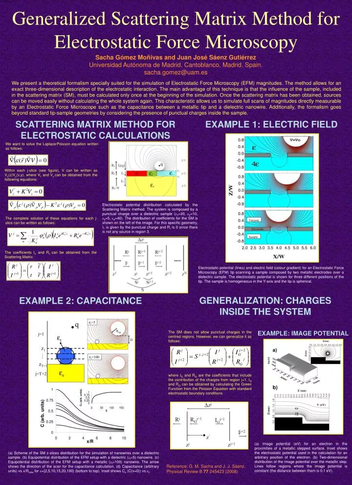
Generalized Scattering Matrix Method for Electrostatic Force Microscopy. Sacha Gómez Moñivas and Juan José Sáenz Gutiérrez Universidad Autónoma de Madrid. Cantoblanco, Madrid. Spain. sacha.gomez@uam.es.

E N D
Generalized Scattering Matrix Method for Electrostatic Force Microscopy Sacha Gómez Moñivas and Juan José Sáenz Gutiérrez Universidad Autónoma de Madrid. Cantoblanco, Madrid. Spain. sacha.gomez@uam.es We present a theoretical formalism specially suited for the simulation of Electrostatic Force Microscopy (EFM) magnitudes. The method allows for an exact three-dimensional description of the electrostatic interaction. The main advantage of this technique is that the influence of the sample, included in the scattering matrix (SM), must be calculated only once at the beginning of the simulation. Once the scattering matrix has been obtained, sources can be moved easily without calculating the whole system again. This characteristic allows us to simulate full scans of magnitudes directly measurable by an Electrostatic Force Microscope such as the capacitance between a metallic tip and a dielectric nanowire. Additionally, the formalism goes beyond standard tip-sample geometries by considering the presence of punctual charges inside the sample. SCATTERING MATRIX METHOD FOR ELECTROSTATIC CALCULATIONS EXAMPLE 1: ELECTRIC FIELD We want to solve the Laplace/Poisson equation written as follows: Within each j-slice (see figure), V can be written as Vz(z)Vr(x,y), where Vz and Vr can be obtained from the following equations: Electrostatic potential distribution calculated by the Scattering Matrix method. The system is composed by a punctual charge over a dielectric sample (e1=20, e2=10, e3=5, e4=40). The distribution of coefficients for the SM is shown on the left of the image. For this specific geometry, I1 is given by the punctual charge and R3 is 0 since there is not any source in region 3. The complete solution of these equations for each j-slice can be written as follows: The coefficients In and Rn can be obtained from the Scattering Matrix: Electrostatic potential (lines) and electric field (colour gradient) for an Electrostatic Force Microscopy (EFM) tip scanning a sample composed by two metallic electrodes over a dielectric sample. The electrostatic potential is shown for three different positions of the tip. The sample is homogeneous in the Y-axis and the tip is spherical. GENERALIZATION: CHARGES INSIDE THE SYSTEM EXAMPLE 2: CAPACITANCE EXAMPLE: IMAGE POTENTIAL The SM does not allow punctual charges in the centred regions. However, we can generalize it as follows: where IG and RG are the coefficients that include the contribution of the charges from region j+1. IG and RG can be obtained by calculating the Green Function from the Poisson Equation with standard electrostatic boundary conditions (a) Image potential (eV) for an electron in the proximities of a metallic stepped surface. Inset shows the electrostatic potential used in the calculation for an arbitrary position of the electron. (b) Two-dimensional distribution of the image potential over the metallic step. Lines follow regions where the image potential is constant (the distance between them is 0.1 eV). (a) Scheme of the SM z-slices distribution for the simulation of nanowires over a dielectric sample. (b) Equipotential distribution of the EFM setup with a dielectric (et=5) nanowire. (c) Equipotential distribution of the EFM setup with a metallic (et=100) nanowire. The arrow shows the direction of the scan for the capacitance calculation. (d) Capacitance (arbitrary units) vs x/Rtube for e={2,5,10,15,20,100} (bottom to top). Inset shows Co (C(x=0)) vs et. Reference: G. M. Sacha and J. J. Sáenz. Physical Review B 77 245423 (2008)