Download
1 / 28
410 likes | 1.86k Views
US Army Corps of Engineers Hydrologic Engineering Center. River Mechanics and Introduction to Unsteady Flow Equations. Objective : Present key items for switching from HEC-RAS steady flow analysis to HEC-RAS unsteady flow simulation. Michael Gee, Ph.D, PE Senior Hydraulic Engineer.

E N D
US Army Corps of Engineers Hydrologic Engineering Center River Mechanics and Introduction to Unsteady Flow Equations • Objective: Present key items for switching from HEC-RAS steady flow analysis to HEC-RAS unsteady flow simulation. Michael Gee, Ph.D, PE Senior Hydraulic Engineer
Steady vs. Unsteady • Difference in handling friction and other losses • Difference in numerical solution algorithm • Difference in computation of X-Sec properties • Difference in handling non-flow areas • Difference in flow and boundary condition data requirements • Difference in calibration strategy • Difference in application strategy
Energy Principles he Energy Grade Line Water Surface Y2 Channel Bottom Y1 Z2 Z1 Datum
Momentum Equation Fx = m a 2 1 P2 W Wx Ff P1 L Z2 Z1 Datum
Momentum Equation P2 - P1 + Wx - Ff = Q Δ Vx Where: P = Hydrostatic Pressure Wx = Force due to weight of water in X direction Ff = Force due to external friction from 2 to 1 Q = Discharge = Density of water Δ Vx = Change in velocity from 2 to 1 in X direction
Momentum Equation – Forces Pressure: Weight: Friction: Where: Mass x acceleration:
Energy vs. Momentum • Energy – Internal energy dissipation represented by loss term, Sf (Manning’s n) • Momentum – External boundary shear forces represented by friction term, Sf (Manning’s n)
Unsteady Flow Equations Momentum Equation: Continuity Equation:
Steady Flow Equations Energy (momentum) Equation: Continuity Equation:
Numerical Solution Friction slope averaging - Steady: Average conveyance Unsteady: Average friction slope
Average conveyance Eq. Average friction slope Eq.
Numerical Solution Algorithms used - Steady: Iterative convergence section-by-section for each flow. Unsteady: Matrix solution for flow and stage simultaneously at all sections each time step.
Numerical Solution of the Unsteady Flow Equations CONVERGENCE The state of tending to a unique solution. A given scheme is convergent if an increasingly finer computational grid leads to a more accurate solution. STABILITY (NUMERICAL or COMPUTATIONAL) The ability of a scheme to control the propagation or growth of small perturbations introduced in the calculations. A scheme is unstable if it allows the growth of error to eventually obliterate the true solution. Ref: River Hydraulics EM
Courant Number For best results, the Cr should be near 1.0
Courant Number Example • Depth ~ 10 ft. • Cross section spacing (x) of ~ 1000 ft. • Requires computational time step (t) about 1 minute
Finite Difference Modeling Considerations • Stability of the computations. • 2. Numerical accuracy of the computations. • 3. Resolution of input hydrographs.
Pre-Computation of Hydraulic Properties(CSECT or HTAB) Steady – Compute exact hydraulic properties at a section for each trial water surface elevation from the GR points, n-values,etc. Unsteady – Hydraulic properties are pre-computed for all possible water surface elevations at each cross section (HTAB)
Non-Flow Areas Steady – “ineffective” areas may or may not be occupied by water. Unsteady – All areas containing water (even if not moving) must be included.
Expansion/Contraction Coeffs. • Not used in the momentum formulation (RAS-unsteady) • Should be in the data, however, for use with steady flow analysis
Data Requirements(Flow and Boundary Conditions) Steady: Discharge (Q) at each cross section. Unsteady: Inflow hydrograph(s) which are routed by the model.
Calibration Strategy – Targets Steady: Match observed water surface (or EGL) elevations. Unsteady: As above, along with timing, hydrograph shape, computed flow distribution in networks.
Calibration Strategy - Adjustments Steady: Manning’s n Unsteady: nand volume (storage); make adjustments throughout range of flows in hydrograph. Add/subtract flows if necessary.
Q Inflow Observed Observed outflow 1 outflow 2 Computed outflow Time Flow Accounting
Application Strategy • 1. Check with range of steady flows • Rough stage calibration. • Possible supercritical flow locations. • Modeling of hydraulic structures.
2. Prepare hydrographs (boundary conditions) Upstream flows Tributary (local flows) Ungaged/unmodeled flows Downstream (rating curve?)
3. Calibration Manning’s n affects both stage and timing. Storage areas can be very important. Fine tuning via conveyance adjustment.