Download
1 / 33
330 likes | 556 Views
Introductory Control Theory. Control Theory. The use of feedback to regulate a signal. Desired signal x d. Controller. Control input u. Signal x. Plant. Error e = x-x d (By convention, x d = 0). x’ = f(x,u). What might we be interested in?. Controls engineering

E N D
Control Theory • The use of feedback to regulate a signal Desired signal xd Controller Control input u Signal x Plant Error e = x-xd (By convention, xd = 0) x’ = f(x,u)
What might we be interested in? • Controls engineering • Produce a policy u(x,t), given a description of the plant, that achieves good performance • Verifying theoretical properties • Convergence, stability, optimality of a given policy u(x,t)
Agenda • PID control • LTI multivariate systems & LQR control • Nonlinear control & Lyapunov funcitons
PID control • Proportional-Integral-Derivative controller • A workhorse of 1D control systems
Proportional term Gain • u(t) = -Kp x(t) • Negative sign assumes control acts in the same direction as x x t
Integral term Integral gain • u(t) = -Kp x(t) - KiI(t) • I(t) = 0tx(t) dt (accumulation of errors) x t Residual steady-state errors driven asymptotically to 0
Instability • For a 2nd order system (momentum), P control Divergence x t
Derivative term Derivative gain • u(t) = -Kp x(t) – Kd x’(t) x
Putting it all together • u(t) = -Kp x(t) - KiI(t) + Kd x’(t) • I(t) = 0tx(t) dt
Example: Damped Harmonic Oscillator • Second order time invariant linear system, PID controller • x’’(t) = A x(t) + B x’(t) + C + D u(x,x’,t) • For what starting conditions, gains is this stable and convergent?
Stability and Convergence • System is stable if errors stay bounded • System is convergent if errors -> 0
Example: Damped Harmonic Oscillator • x’’ = A x + B x’ + C + D u(x,x’) • PID controller u = -Kp x –Kd x’ – Ki I • x’’ = (A-DKp) x + (B-DKd) x’ + C - D Ki I
Homogenous solution • Instable if A-DKp > 0 • Natural frequency w0 = sqrt(DKp-A) • Damping ratio z=(DKd-B)/2w0 • If z > 1, overdamped • If z < 1, underdamped (oscillates)
Multivariate Systems • x’ = f(x,u) • x X Rn • u U Rm • Because m n, and variables are coupled, this is not as easy as setting n PID controllers
Linear Time-Invariant Systems • Linear: x’ = f(x,u,t) = A(t)x + B(t)u • LTI: x’ = f(x,u) = Ax + Bu • Nonlinear systems can sometimes be approximated by linearization
Convergence of LTI systems • x’ = A x + B u • Let u = - K x • Then x’ = (A-BK) x • The eigenvaluesli of (A-BK) determine convergence • Each li may be complex • Must have real component between (-∞,0]
Linear Quadratic Regulator • x’ = Ax + Bu • Objective: minimize quadratic cost xTQ x + uTR u dtOver an infinite horizon Error term “Effort” penalization
Closed form LQR solution • Closed form solutionu = -K x, with K = R-1BP • Where P solves the Riccati equation • ATP + PA – PBR-1BTP + Q = 0 • Derivation: calculus of variations
Solving Riccati equation • Solve for P inATP + PA – PBR-1BTP + Q = 0 • Existing iterative techniques, e.g. in Matlab
Nonlinear Control • x’ = f(x,u) • How to find u? • Next class • How to prove convergence and stability? • Hard to do across X
Proving convergence & stability with Lyapunov functions • Let u = u(x) • Then x’ = f(x,u) = g(x) • Conjecture a Lyapunov function V(x) • V(x) = 0 at origin x=0 • V(x) > 0 for all x in a neighborhood of origin V(x)
Proving stability with Lyapunov functions • Idea: prove that d/dt V(x) 0 under the dynamics x’ = g(x) around origin V(x) t g(x) t d/dt V(x)
Proving convergence with Lyapunov functions • Idea: prove that d/dt V(x) < 0 under the dynamics x’ = g(x) around origin V(x) t g(x) t d/dt V(x)
Proving convergence with Lyapunov functions • d/dt V(x) = dV/dx(x) dx/dt(x) = V(x)T g(x) < 0 V(x) t g(x) t d/dt V(x)
How does one construct a suitable Lyapunov function? • It may not be easy… • Typically some form of energy (e.g., KE + PE)
Handling Uncertainty • All the controllers we have discussed react to disturbances • Some systems may require anticipating disturbances • To be continued…
Motion Planning and Control • Replanning = control?
Motion Planning and Control • Replanning = control? PRM planning Real-time planning Optimal control Model predictive control Reactive Control Accurate models Coarse models Explicit plans computed Policies engineered Computationally expensive Computationally cheap
Planning or control? • The following distinctions are more important: • Tolerates disturbances and modeling errors? • Convergent? • Optimal? • Scalable? • Inexpensive?
Presentation Schedule • Optimal Control, 3/30 • Ye and Adrija • Operational space and force control, 4/1 • Yajia and Jingru • Learning from demonstration, 4/6 • Yang, Roland, and Damien • Planning under uncertainty, 4/8 • You Wei and Changsi • Sensorless planning, 4/13 • Santhosh and Yohanand • Planning to sense, 4/15 • Ziaan and Yubin