Download

1 / 38
380 likes | 652 Views
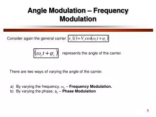
ANGLE MODULATION (AM). Part 1 Introduction. Objectives. To define and explain frequency modulation (FM) and phase modulation (PM) To analyze the FM in terms of Mathematical analysis To analyze the Bessel function for FM and PM To analyze the FM bandwidth and FM power distribution.

E N D
ANGLE MODULATION(AM) Part 1 Introduction
Objectives • To define and explain frequency modulation (FM) and phase modulation (PM) • To analyze the FM in terms of Mathematical analysis • To analyze the Bessel function for FM and PM • To analyze the FM bandwidth and FM power distribution
Lecture overview • Frequency modulation (FM) and phase modulation (PM) • Analysis of FM • Bessel function for FM and PM • FM bandwidth • Power distribution of FM
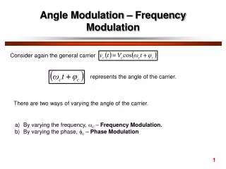
Introduction • Angle modulation is the process by which the angle (frequency or Phase) of the carrier signal is changed in accordance with the instantaneous amplitude of modulating or message signal. • also known as “Exponential modulation"
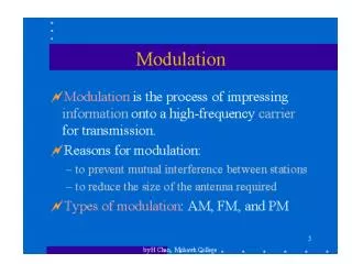
Cont’d… • classified into two types such as • Frequency modulation (FM) • Phase modulation (PM) • Used for : • Commercial radio broadcasting • Television sound transmission • Two way mobile radio • Cellular radio • Microwave and satellite communication system
Frequency Modulation (FM)Introduction • FM is the process of varying the frequency of a carrier wave in proportion to a modulating signal. • The amplitude of the carrier wave is kept constant while its frequency and a rate of change are varied by the modulating signal.
FM :Introduction (cont…) • Fig 3.1 : Frequency Modulated signal
FM :Introduction (cont…) • The important features about FM waveforms are : • The frequency varies. • The rate of change of carrier frequency changes is the same as the frequency of the information signal. • The amount of carrier frequency changes is proportional to the amplitude of the information signal. • The amplitude is constant.
FM :Introduction (cont…) • The FM modulator receives two signals,the information signal from an external source and the carrier signal from a built in oscillator. • The modulator circuit combines the two signals producing a FM signal which passed on to the transmission medium. • The demodulator receives the FM signal and separates it, passing the information signal on and eliminating the carrier signal. • Federal Communication Coporation (FCC) allocation for a standard broadcast FM station is as shown in Fig.3.2
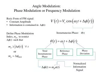
Analysis of FM • Mathematical analysis: • Let message signal: • (3.1) • And carrier signal: (3.2) • Where carrier frequency is very much higher than message frequency.
Analysis of FM (cont’d) • In FM, frequency changes with the change of the amplitude of the information signal. So the instantenous frequency of the FM wave is; • (3.3) • K is constant of proportionality
Analysis of FM(cont’d) • Thus, we get the FM wave as: (3.4) • Where modulation index for FM is given by
Analysis of FM(cont’d) • Frequency deviation: ∆f is the relative placement of carrier frequency (Hz) w.r.t its unmodulated value. Given as:
FM(cont’d) • Therefore:
Example 3.1 • FM broadcast station is allowed to have a frequency deviation of 75 kHz. If a 4 kHz (highest voice frequency) audio signal causes full deviation (i.e. at maximun amplitude of information signal) , calculate the modulation index.
Example 3.2 • Determine the peak frequency deviation, , and the modulation index, mf, for an FM modulator with a deviation Kf = 10 kHz/V. The modulating signal to be transmitted is Vm(t) = 5 cos ( cos 10kπt).
FM&PM (Bessel function) • Thus, for general equation:
B.F. (cont’d) • It is seen that each pair of side band is preceded by J coefficients. The order of the coefficient is denoted by subscript m. The Bessel function can be written as • N=number of the side frequency • M=modulation index
BesselFunctions of the First Kind, Jn(m) for some value of modulation index
FM Bandwidth • Theoretically, the generation and transmission of FM requires infinite bandwidth. Practically, FM system have finite bandwidth and they perform well. • The value of modulation index determine the number of sidebands that have the significant relative amplitudes • If n is the number of sideband pairs, and line of frequency spectrum are spaced by fm, thus, the bandwidth is: • For n=>1
Cont’d… • Estimation of transmission b/w; • Assume mf is large and n is approximate mf +2; thus • Bfm=2(mf +2)fm = (1) is called Carson’s rule
Deviation ratio (DR) • The worse case modulation index which produces the widest output frequency spectrum. • Where • ∆f(max) = max. peak frequency deviation • fm(max) = max. modulating signal frequency
Example 3.3 An FM modulator is operating with a peak frequency deviation =20 kHz.The modulating signal frequency, fm is 10 kHz, and the 100 kHz carrier signal has an amplitude of 10 V. Determine : a) The minimum bandwidth using Bessel Function table. b)The minimum bandwidth using Carson’s Rule. c)Sketch the frequency spectrum for (a), with actual amplitudes.
Example 3.4 For an FM modulator with a modulation index m=1, a modulating signal Vm(t)=Vm sin(2π1000t), and an unmodulated carrier Vc(t) = 10sin(2π500kt), determine : a) Number of sets of significant side frequencies b) Their amplitudes c) Draw the frequency spectrum showing their relative amplitudes.
Example 3.4 (solution) a) From table of Bessel function, a modulation index of 1 yields a reduced carrier component and three sets of significant side frequencies. b) The relative amplitude of the carrier and side frequencies are • Jo = 0.77 (10) = 7.7 V • J1 = 0.44 (10) = 4.4 V • J2 = 0.11 (10) = 1.1 V • J3 = 0.02 (10) = 0.2 V
7.7 V 4.4V 4.4V 1.1V 1.1V 0..2 0..2 Example 3.4 (solution) • Frequency spectrum • 497 498 499 500 501 502 503 • J3 J2 J1 JO J1 J2 J3
FM Power Distribution • As seen in Bessel function table, it shows that as the sideband relative amplitude increases, the carrier amplitude,J0 decreases. • This is because, in FM, the total transmitted power is always constant and the total average power is equal to the unmodulated carrier power, that is the amplitude of the FM remains constant whether or not it is modulated.
Cont’d… • In effect, in FM, the total power that is originally in the carrier is redistributed between all components of the spectrum, in an amount determined by the modulation index, mf, and the corresponding Bessel functions. • At certain value of modulation index, the carrier component goes to zero, where in this condition, the power is carried by the sidebands only.
Average Power • The average power in unmodulated carrier • The total instantaneous power in the angle modulated carrier. • The total modulated power
Example 3.5 • a) Determine the unmodulated carrier power for the FM modulator and condition given in example 3.4, (assume a load resistance RL = 50 Ώ) • b) Determine the total power in the angle modulated wave.
Example 3.5 (solution) • a) Pc = (10)(10)/(2)(50) =1 W • b)
At the end of this chapter, you should be able, • To define and explain frequency modulation (FM) and phase modulation (PM) • To analyze the FM in terms of Mathematical analysis • To analyze the Bessel function for FM and PM • To analyze the FM bandwidth and FM power distribution