Download
1 / 60
600 likes | 749 Views
Optical Solutions for Bounded NP-Complete Problems. Shlomi Dolev joint work with: Hen Fitoussi, Ephraim Korach, Stephane Messika, Yuval Nir, Yossi Rosen, Natan Shaked, Galit Uzan Ben-Gurion University of the Negev. Optical Computing, Now?. Optical computing mature enough (Bell Labs, NASA,…)

E N D
Optical Solutions for Bounded NP-Complete Problems Shlomi Dolev joint work with: Hen Fitoussi, Ephraim Korach, Stephane Messika, Yuval Nir, Yossi Rosen, Natan Shaked, Galit Uzan Ben-Gurion University of the Negev
Optical Computing, Now? • Optical computing • mature enough (Bell Labs, NASA,…) and • young enough (Optical Switches) to make the right decisions concerning the architecture of optical processors • Advances in optical switches • computers are built with switching elements • The applications of such inherently parallel devices are enormous and may change the entire world of computers
Optical Computing, Now? • Moore Law is brokenno more doubling of the number of transistors every 18 months • MultiCore? Maybe each light beam is a core? • Avoid (fiber) Optics to Electronics and back
Applications • Cryptologic Quarterly NSA- Top Secret 1982-96 publication declassified- Indicates a great interest in optics for cryptographic use • Quantum Computing, yet to be implemented, and limited • Combinatorial Optimization Problems
Talk Overview The traveling beams [DN, 2006] U.S. Patent Vector Matrix based architectures [SMDR 2007] Applied Optics [STSMDR 2007] Optical Engineering Coordinated Holes Masks-Made-Black Box [DF 2007] FUN with Algorithms
Exhaustive Search? Why not approximation or heuristic methods? • Approximation methods: • Preferring good solutions found quicklyrather than the best one which may not be found within reasonable time. • Heuristic methods: • Solving the problem quickly for certain cases only. • The computation time of the heuristic methods may be unexpected and even longer than that of an exhaustive search due to unsuccessful attempts for optimization. • Therefore,in applications wheredeadlines must be met, the proposed optical method can provide adramatically betterguarantied time for the solution(compared to the exhaustive search electronic solution).
Inherent Parallelism for Hard Computing Problems • Enables us to use new approaches for coping with NP-complete problems • Designing primitives for TSP/Hamiltonian-Path proposed in U.S. Patent [Dolev and Nir, 2006] • Implementation of a micro-processor for the Hamiltonian-Path problem
A new 3D Architecture for Optical Processor Vertex 2 Vertex 3 Vertex 1
Optical Processor Architecture • Information transfer between the elements is performed by propagating light in free space, in parallel • The location the beam reaches represents the (current) computation result
Vertex 1 Vertex 3 Vertex 2 Optical Processor (Graph Based) Architecture The Columns The Graph
Optical Processor Architecture • Each column is mapped to a group of states that share a specific attribute • The graph locations are mapped to each vertex • Programmable mask will block the light between nodes that are not connected
Hamiltonian-Path Architecture Vertex 2 Eachlocation represents a path Vertex 3 Vertex 1
Hamiltonian Path - Architecture Vertex 2 Mask is used to block unfeasible paths Vertex 3 Vertex 1
Hamiltonian Path - Architecture Vertex 2 Vertex 3 Vertex 1
Hamiltonian Path - Architecture Vertex 2 Light in the last layer indicates the existence of Hamiltonian-path 1 2 3 Vertex 1 Vertex 3
Vertex 2 Vertex 1 Vertex 3 Hamiltonian-path • V1 →V3 →V2 • V1 →V3 →V1 Level 3
Experimental Demonstration • Small problem: 3 nodes • 10mW HeNe laser as the input light source • For splitting the light: • 2 refractive beam splitters in each vertex • 2 × 3 = 6 refractive beam splitters in the entire system • Future implementations will probably use diffractive elements as beam splitters • For redirecting the light between vertices: • 2 mirrors in each edge • 2 × 3 = 6 mirrors for the entire system • No amplification in small problem solutions • For the solution of bigger problems, an optical amplification will have to be used
Other Basic Primitives Polynomial reductions? 3-Sat, 3D Matching, Vertex Cover, Clique, Partition, Independent Set Instead of add, sub, xor… #P problems, Permanent
Partition Input: a set S of n integers {a1, a2, a3, …, an} Output: a partition of S into 2 disjoint sets S1 and S2 such that Σ S1 = Σ S2
Partition Architecture LightSource a1 a2 a3 {a1, a2, a3} {a1, a2} Lens Detector
Talk Overview The traveling beams [DN, 2006] U.S. Patent Vector Matrix based architectures [SMDR 2007] Applied Optics [STSMDR 2007] Optical Engineering Coordinated Holes Masks-Made-Black Box [DF 2007] FUN with Algorithms
Tour Lengths Binary Matrix Weight Vector = Example:N = 4 w12 w14 1 l1 w13 w12 1 4 = l2 w24 0 = [( - 1)! /2] = 3 N [( - 1)! /2] 3 N w13 w23 1 1 w34 l3 2 1 1 w14 0 w23 0 3 0 1 [ N ( N 1)/2]=6 - 0 w24 1 1 1 1 w34 1 = N N 1)/2] ( - 6 [ 1 0 Solving the TSP/HPP by an Optical Vector-Matrix Multiplication (VMM) • The power of optics in this TSP/HPP solver is realized by using a fastoptical vector-matrix multiplication (VMM): . The minimal element of this vector coincideswith the minimal tour • ANY OPTICAL VECTOR-MATRIX MULTIPLIER CAN BE USED. • Synthesizing the binary-matrix...
Synthesis of the Binary-Matrix The binary-matrix synthesis is regarded as apreprocessing. Eachcolumn represents a directededge(or weight wij). Eachrow represents afeasible tour: . … … … ‘1’ in row r and column c means that the salesman passes through the edge c in the tour Tr 1 …
Synthesis of the Binary-Matrix • Initialization:Start from thebinary-matrix of N=3 nodes(containing only two tours). • Transition: • Define an [(N−1)!]×[N(N−1)+1] target matrix. • Divide the target matrix into (N−1) horizontal sections. • Duplicate each columnfrom the the source matrix into the target matrix by changing its indices according to a well-defined set of rules. • Fill the unfilled positions in the target matrix with zeros. Target matrix:N-node binary-matrix Source matrix:(N−1)-node binary-matrix From 3 to 4 Cities…
Inside the mask for N = 6, we can see the mask for N = 5 Synthesis of the Binary-Matrix ~N = 3 ~N = 4 ~N = 5 N = 6
Synthesis of the Binary-Matrix Advantagesof the New Algorithm • Aftersynthesizing the binary-matrix once– all TSPs and HPPs of the same degree or less (N or fewer nodes) can be solved using the same binary-matrix. • Only O(N3) duplicationsof big vectors (in the size of O(N!)). • Can be implemented in anoptical way.
Optical Synthesis of the Binary-Matrix • Thevector duplicationsare done bycorrelating shifted point (delta) functionsby each of the source matrix columns. • The delta functionsshifts are given by the binary-matrix algorithm. Source matrix:(N−1)-node binary-matrix Target matrix:N-node binary-matrix O(N2) vector duplications. Size of each vector: O(N!)
Duplication Using the 4f Optical System Transformed Delta Functions N=4 Binary-Matrix N=5 Binary-Matrix f f f f y fy fx Plane Wave x u v P2 P1 P3 L1 L2 Input Plane Filter Plane Output Plane
PC for the CCD Camera (Output Plane) Fourier Transform Lens (L2) Fourier Transform Lens (L1) PC for the SLM (Filter Plane) Polarized Laser SLM and Analyzer CCD Camera Mirror Input Plane Beam Expander Shutter Mirror Binary Matrix Synthesizer Electro-Optics Laboratory, BGUApril 2006
Simulation and Experimental Results Optical Synthesis of the N=5 Binary-Matrix Experimental Results Simulation Results
800 1 2 100 1 900 50 190 250 130 15 100 600 20 300 200 5 3 150 800 500 30 30 400 4 100 5-Node TSP Example BEST TOUR: 13245 L = w13+w32+w24+w45+w51
VMM by the 4f Optical System Transformation of the Binary-Matrix Grayscale Weight-Vector Correlation Matrix f f f f fy y fx u Plane Wave x v P1 P2 P3 L2 L1 Input Plane Filter Plane Output Plane
Best Route ref w12 w13 w14 w15 w21 w23 w24 w25 w32 w31 w34 w35 w42 w43 w41 w45 w52 w53 w54 w51 1 2 1 w13+w24+w32+w45+w51 BEST TOUR: 13245 5 3 4
5 10 Optical Processor Electronic Processor 0 10 5- Logarithmic Axis: Computation Time (seconds) 10 10- 10 15- 10 3 4 5 6 7 8 9 10 11 12 13 14 15 16 Number of TSP cities Comparison between the computation times of the optical and electronic processors for solving various TSPs (after the binary-matrix is already synthesized in the preprocessing by the new efficient algorithm)
Talk Overview The traveling beams [DN, 2006] U.S. Patent Vector Matrix based architectures [SMDR 2007] Applied Optics [STSMDR 2007] Optical Engineering Coordinated Holes Masks-Made-Black Box [DF 2007] FUN with Algorithms
The Black BoxArchitecture • A set of masks is created according to the problem • A subset of this set is chosen according to the input
The Black BoxArchitecture The number of beams reached the detector determines the output Lens Detector
Hamiltonian-cycle • Each edge is represented by a mask (opaque/transparent screen) • A mask will represent all possible Hamiltonian-paths • The mask of ei is transparent if ei not in the path, and opaque otherwise
The Masks The mask is transparent if ei is not in path, and opaque otherwise e3 →e2 →e4 • n! locations in a mask • n2 masks e3 →ei →e4
V1 e12 V2 e31 e23 V3 Example Given an input graph
V1 e21 V2 e31 e23 V3 Example Asubset of the masks is chosen according to the input graph e31 e23 e21 e32 Lens Detector e13 e12
Why Does it Work? P = e12 →e23 →e31 V1 e21 e12 V2 e31 e23 V3
Why Does it Work? P = e12 →e23 →e31 V1 e12 V2 e31 e23 V3
Creating the Mask • The mask is created using an optical copying algorithm [SSTMDR07] • The initial mask is a mask of three vertices
The Idea e12 V1 V2 e31 e23 V3
The Idea V1 V2 e12 e23 V1 e42 V3 e31 V2 e34 e23 V4 V3
V1 V2 e23 V3 e34 V4 The Idea V1 V2 e21 V3 e42 e34 V4
Creating the Masks N=3 N=4