Download
1 / 16
280 likes | 626 Views
NP-Complete Problems. Problems Abstract Problems Decision Problem, Optimal value, Optimal solution Encodings //Data Structure Concrete Problem //Language Class of Problems P NP NP-Complete NP-Completeness Proofs Solving hard problems Approximation Algorithms. Abstract Problems.

E N D
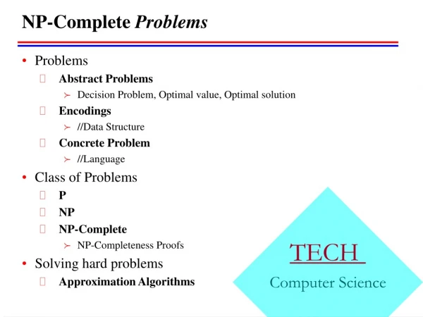
NP-Complete Problems Problems Abstract Problems Decision Problem, Optimal value, Optimal solution Encodings //Data Structure Concrete Problem //Language Class of Problems P NP NP-Complete NP-Completeness Proofs Solving hard problems Approximation Algorithms
Abstract Problems • a formal notion of what a “problem” is • high-level description of a problem • We define an abstract problem Q to be • a binary relation on • a set I of problem instances, and • a set S of problem solutions. • Q I S • Three Kinds of Problems • Decision Problem • e.g. Is there a solution better than some given bound? • Optimal Value • e.g. What is the value of a best possible solution? • Optimal Solution • e.g. Find a solution that achieves the optimal value.
Encodings • // Data Structure • describing abstract problems (for solving by computers) • in terms of data structure or binary strings • An encoding of a set S of abstract objects is • a mapping e from S to the set of binary strings. • Encoding for Decision problems • Problem instances, e : I {0, 1}* • Solution, e : S {0, 1} • “Standard” encoding • computing time may be a function of encoding • // The size of the input (the number of bit to represent one input) • polynomially related encodings • assume encoding in a reasonable concise fashion
Concrete Problem • problem instances and solutions are represented in data structure or binary strings • // Language (in formal-language framework) • We call a problem whose instance set (and solution set) is the set of binary strings a concrete problem. • Computer algorithm solves concrete problems! • solves a concrete problem in time O(T(n)) • if provided a problem instance i of length n = |i|, • the algorithm can produce the solution • in a most O(T(n)) time. • A concrete problem is polynomial-time solvable • if there exists an algorithm to solve it in time O(nk) • for some constant k. (also called polynomially bounded)
Class of Problems • // What makes a problem hard? • // Make simple: classify decision problems • Definition: The class P • P is the class of decision problems that are polynomially bounded. • // there exist a deterministic algorithm • Definition: The class NP • NP is the class of decision problems for which there is a polynomially bounded non-deterministic algorithm. • The name NP comes from “Non-deterministic Polynomially bounded.” • // there exist a non-deterministic algorithm • Theorem: P NP
The Class NP • NP is a class of decision problems for which • a given proposed solution (called certificate) for • a given input • can be checked quickly (in polynomial time) • to see if it really is a solution. • A non-deterministic algorithm • The non-deterministic “guessing” phase. • Some completely arbitrary string s, “proposed solution” • each time the algorithm is run the string may differ • The deterministic “verifying” phase. • a deterministic algorithm takes the input of the problem and the proposed solution s, and • return value true or false • The output step. • If the verifying phase returned true, the algorithm outputs yes. Otherwise, there is no output.
The Class NP-Complete • A problem Q is NP-complete • if it is in NP and • it is NP-hard. • A problem Q is NP-hard • if every problem in NP • is reducible to Q. • A problem P is reducible to a problem Q if • there exists a polynomial reduction function T such that • For every string x, • if x is a yes input for P, then T(x) is a yes input for Q • if x is a no input for P, then T(x) is a no input for Q. • T can be computed in polynomially bounded time.
Polynomial Reductions • Problem P is reducible to Q • P p Q • Transforming inputs of P • to inputs of Q • Reducibility relation is transitive.
Circuit-satisfiability problem is NP-Complete • Circuit-satisfiability problem • belongs to the class NP, and • is NP-hard, i.e. • every problem in NP is reducible to circuit-satisfiability problem! • Circuit-satisfiablity problem • we say that a one-output Boolean combinational circuit is satisfiable • if it has a satisfying assignment, • a truth assignment (a set of Boolean input values) that • causes the output of the circuit to be 1 • Proof…
NP-Completeness Proofs • Once we proved a NP-complete problem • To show that the problem Q is NP-complete, • choose a know NP-complete problem P • reduce P to Q • The logic is as follows: • since P is NP-complete, • all problems R in NP are reducible to P, R p P. • show P p Q • then all problem R in NP satisfy R p Q, • by transitivity of reductions • therefore Q is NP-complete
Solving hard problems:Approximation Algorithms • an algorithm that returns near-optimal solutions • may use heuristic methods • e.g. greedy heuristics • Definition:Approximation algorithm • An approximation algorithm for a problem is • a polynomial-time algorithm that, • when given input I, outputs an element of FS(I). • Definition: Feasible solution set • A feasible solution is • an object of the right type but not necessarily an optimal one. • FS(I) is the set of feasible solutions for I.
Approximation Algorithm e.g. Bin Packing • How to pack or store objects of various sizes and shapes • with a minimum of wasted space • Bin Packing • Let S = (s1, …, sn) • where 0 < si <= 1 for 1 <= i <= n • pack s1, …, sn into as few bin as possible • where each bin has capacity one • Optimal solution for Bin Packing • considering all ways to • partition S into n or fewer subsets • there are more than • (n/2)n/2 possible partitions
Bin Packing: First fit decreasing strategy • places an object in the first bin in which it fits • W(n) in (n2)
Algorithm: Bin Packing (first fit decreasing) • Input: A sequence S=(s1,….,sn) of type float, where 0<si<1 for 1<=i<=n. S represents the sizes of objects {1,...,n} to be placed in bins of capacity 1.0 each. • Output: An array bin where for 1<=i<=n, bin[i] is the number of the bin into which object i is placed.For simplicity,objects are indexed after being sorted in the algorithm.The array is passed in and the algorithm fills it. • binpackFFd(S,n,bin) • float[] used=new float[n+1]; • //used[j] is the amount of space in bin j already used up. • int i,j; • Initialize all used entries to 0.0 • Sort S into descending(nonincreasing)order,giving the sequence s1>=S2>=…>=Sn. • for(i=1;i<=n;i++) • //Look for a bin in which s[i] fits. • for(j=1;j<=n;j++) • if(used[j]+si<+1.0) • bin[i]=j; • used[j] += si; • break; //exit for(j) • //continue for(i).
The Traveling Salesperson Problem • given a complete, weighted graph • find a tour (a cycle through all the vertices) of • minimum weight • e.g.
Approximation algorithm for TSP • The Nearest-Neighbor Strategy • as in Prim’s algorithm … • NearestTSP(V, E, W) • Select an arbitrary vertex s to start the cycle C. • v = s; • While there are vertices not yet in C: • Select an edge vw of minimum weight, where w is not in C. • Add edge vw to C; • v = w; • Add the edge vs to C. • return C; • W(n) in O(n2) • where n is the number of vertices