Download
1 / 33
330 likes | 457 Views
A Simple Model for Oxygen Dynamics in Chesapeake Bay. Malcolm Scully. Center for Coastal Physical Oceanography. Old Dominion University. Center for Coastal Physical Oceanography. Community Surface Dynamics Modeling System (CSDMS) 2011 Meeting; Boulder, CO. Outline:.

E N D
A Simple Model for Oxygen Dynamics in Chesapeake Bay Malcolm Scully Center for Coastal Physical Oceanography Old Dominion University Center for Coastal Physical Oceanography Community Surface Dynamics Modeling System (CSDMS) 2011 Meeting; Boulder, CO Outline: • Background and Motivation • Simplified Modeling Approach • Importance of Physical Forcing to Seasonal Variations in Hypoxic Volume • River Discharge • Heat Flux / Temperature • Wind (Magnitude and Direction) • Inter-annual Variation in Hypoxic Volume • Conclusions
Testbed to Improve Models of Environmental Processes on the U.S. Atlantic and Gulf of Mexico Coasts Estuarine Hypoxia Team • Federal partners • David Green (NOAA-NWS) – Transition to operations at NWS • Lyon Lanerole, Rich Patchen, Frank Aikman (NOAA-CSDL) – Transition to operations at CSDL; CBOFS2 • Lewis Linker (EPA), Carl Cerco (USACE) – Transition to operations at EPA; CH3D, CE-ICM • Doug Wilson (NOAA-NCBO) – Integration w/observing systems at NCBO/IOOS • CSDMS partners • Carl Friedrichs (VIMS) – Project Coordinator • Marjorie Friedrichs, Aaron Bever (VIMS) – Metric development and model skill assessment • Ming Li, Yun Li (UMCES) – UMCES-ROMS hydrodynamic model • Wen Long, Raleigh Hood (UMCES) – ChesROMS with NPZD water quality model • Scott Peckham, JisammaKallumadikal (UC-Boulder) – Running multiple models on a single HPC cluster • Malcolm Scully (ODU) – ChesROMS with 1 term oxygen respiration model • Kevin Sellner (CRC) – Academic-agency liason; facilitator for model comparison • JianShen (VIMS) – SELFE, FVCOM, EFDC models
ChesROMS and two other flavors of ROMS are already incorporated into CSDMS. 1) Run CSDMS Modeling Tool 2) “File” “Open Project” “Marine” “ROMS” 3) Drag selected “Palette” (“chesROMS” in this case) into Driver; 4) Choose “Configure”, adjust settings as desired; 5) Run chesROMS
Map of Mean Bottom Dissolved Oxygen -- Summer 2005 • Low DO has significant impact on a wide array of biological and ecological processes. • Large regions of Chesapeake Bay are impacted by hypoxia/anoxia. • Over $ 3.5 billion was spent on nutrient controls in Chesapeake Bay between 1985-1996 (Butt & Brown, 2000) • Assessing success/failure of reductions in nutrient loading requires understanding of the physical processes that contribute to the inter-annual variability. From Chesapeake Bay Program newsletter: http://ian.umces.edu/pdfs/do_letter.pdf
Regional Ocean Modeling System (ROMS) • Model forcing • Realistic tidal and sub-tidal elevation at ocean boundary • Realistic surface fluxes from NCEP (heating and winds) • Observed river discharge for all tributaries. • Temperature and salinity at ocean boundary from World Ocean Atlas. ChesROMS Model Grid
Depth-dependent Respiration Formulation • Oxygen Model • Oxygen is introduced as an additional model tracer. • Oxygen consumption (respiration) is constant in time, with depth-dependent vertical distribution. • No oxygen consumption outside of estuarine portion of model • No oxygen production. • Open boundaries = saturation • Surface flux using wind speed dependent piston velocity following Marino and Howarth, 1993. • No negative oxygen concentration and no super-saturation. Surface Oxygen Flux using Piston Velocity: Model assumes biology is constant so that the role of physical processes can be isolated! From Marino and Howarth, Estuaries, 1993
Seasonal and Inter-Annual Variability in Hypoxic Volume (from CBP data 1984-2009) Maximum observed Minimum observed Data compiled from Murphy et al. (submitted)
Variability of Physical Forcing What is relative importance of different physical forcing in controlling seasonal and inter-annual variability of hypoxia in Chesapeake Bay?
Comparison with Bottom DO at Chesapeake Bay Program Stations
Comparison with Chesapeake Bay Program Data Bottom Dissolved Oxygen Concentration (mg/L) July 19-21, 2004 August 9-11, 2004
In addition to seasonal cycle, model captures some of the inter-annual variability 707 km3days 485 km3days 476 km3days Model predicts roughly 50% more hypoxia in 2004 than in 2005, solely due to physical variability.
Physical Controls on Hypoxia in Chesapeake Bay Malcolm Scully Center for Coastal Physical Oceanography Old Dominion University Center for Coastal Physical Oceanography Virginia Institute of Marine Sciences, Seminar October 21, 2011 Outline: • Background and Motivation • Simplified Modeling Approach • Importance of Physical Forcing to Seasonal Variations in Hypoxic Volume • River Discharge • Heat Flux / Temperature • Wind (Magnitude and Direction) • Inter-annual Variation in Hypoxic Volume • Conclusions
River Discharge Monthly Climatology Susquehanna River at Conowingo Dam (1967-2010) m3/s Month
Importance of Seasonal Variations in River Flow Hypoxic Volume (< 1 mg/L) 2004
Sensitivity to River Discharge Hypoxic Volume (< 1 mg/L) Integrated volumes: 469 km3days 488 km3days 476 km3days 423 km3days Order of magnitude change in river discharge leads to less than 10% change in integrated hypoxic volume. 2004
Water Temperature Monthly climatology at Thomas Point Light (1986-2009)
To simulate realistic variability in temperature forcing, model was run changing the air temperature by ± one standard deviation based on monthly climatology for air temperature. Bay-averaged Water Temp (model) Thomas Point Light Water Temp 1998 + 1 std air temp 1992 - 1 std air temp
Sensitivity to Temperature Hypoxic Volume (< 1 mg/L) Integrated volumes: + 1 std air temp - 1 std air temp 421km3days 534 km3days Increase in surface heating results in greater than 20% change in integrated hypoxic volume. 2004
Wind Forcing Wind Climatology from Thomas Point Light (1986-2010) a) Wind Speed b) Wind Direction m/s
Importance of Seasonal Variations in Wind Hypoxic Volume (< 1 mg/L) 2004
To simulate realistic variability in wind forcing, May-August wind magnitudes were increased/decreased by 15%. Average Monthly Wind Speed from Model Mid-Bay location
Sensitivity to Wind Speed Hypoxic Volume (< 1 mg/L) Integrated volumes: 751 km3days 476 km3days 242 km3days Realistic changes in summer wind speed could change hypoxic volume by a factor of 3 2004
Sensitivity to Summer Wind Direction Modeled summer wind direction Positive 90° Base Summer Winds Negative 90° 180°
Sensitivity to Summer Wind Direction Hypoxic Volume (< 1 mg/L) Integrated volumes: 548 km3days 527 km3days 476 km3days 278 km3days Changes in wind direction can change the hypoxic volume by a factor of 2 2004
Physical Controls on Hypoxia in Chesapeake Bay Malcolm Scully Center for Coastal Physical Oceanography Old Dominion University Center for Coastal Physical Oceanography Virginia Institute of Marine Sciences, Seminar October 21, 2011 Outline: • Background and Motivation • Simplified Modeling Approach • Importance of Physical Forcing to Seasonal Variations in Hypoxic Volume • River Discharge • Heat Flux / Temperature • Wind (Magnitude and Direction) • Inter-annual Variation in Hypoxic Volume • Conclusions
Analysis of 15-year Simulation of Hypoxic Volume (1991-2005) Bi-monthly Averages Observations Model max Hypoxic Volume (<1mg/L) Hypoxic Volume (<1mg/L) mean min month month Model with no biologic variability shows significant inter-annual variability Observations have greater variability than model Model under predicts in early summer and slightly over predicts in late summer
Does variation in physical forcing explain observed inter-annual variability in hypoxic volume? r = 0.32 p = 0.25 Not in a statistically significant way! Annual Mean Hypoxic Volume (Modeled) Annual Mean Hypoxic Volume (Observed)
Next Steps: Simplified Load-Dependent Respiration Rate Monthly-averaged Respiration Rate Load-Dependent Respiration Rate (Scaled by Integrated Nitrogen Loading—Previous 250 days)
Preliminary Results with Load-Dependent Respiration Rate Constant Resp. Rate Load-dependent Resp. Rate r = 0.315 p =0.252 r = 0.628 p =0.016 Hypoxic Volume (Modeled) Hypoxic Volume (Modeled) Hypoxic Volume (Observed) Hypoxic Volume (Observed)
Conclusions • A relatively simple model with no biological variability can reasonably account for the seasonal cycle of hypoxia in Chesapeake Bay. • Wind speed and direction are the two most important physical variables controlling hypoxia in the Bay. • Model results are largely insensitive to variations in river discharge, when the role of nutrient delivery is not accounted for. • Changes in air temperature and the associated changes in water temperature via sensible heat flux can have a measurable influence on the overall hypoxic volume. • A 15-year model simulation with constant respiration rate produces significant inter-annual variability in hypoxic volume, by largely fails to reproduce the observed variability. • Model residuals are significantly correlated with the integrated Nitrogen loading demonstrating the importance of biological processes in controlling inter-annual variability • Preliminary attempts to include the effects of nutrient loading though a load-dependent respiration formulation show promise for capturing observed inter-annual variability.