Download
1 / 63
630 likes | 808 Views
3.2. Neurons and their networks 3.2.1 Biological neurons. Tasks such as navigation, but also cognition, memory etc. happen in the nervous system (more specifically the brain). The nervous system is made up of several different types of cells: - Neurons - Astrocytes - Microglia

E N D
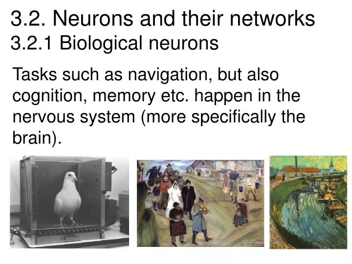
3.2. Neurons and their networks 3.2.1 Biological neurons Tasks such as navigation, but also cognition, memory etc. happen in the nervous system (more specifically the brain).
The nervous system is made up of several different types of cells: - Neurons - Astrocytes - Microglia - Schwann cells Neurons do the computing, the rest is infrastructure
Astrocytes • Star-shaped, abundant, and versatile • Guide the migration of developing neurons • Act as K+ and NT buffers • Involved in the formation of the blood brain barrier • Function in nutrient transfer
Microglia • Specialized immune cells that act as the macrophages of the central nervous system
Schwann cells andOligodendrocytes Produce the myelin sheath which provides the electrical insulation for neurons and nerve fibers Important in neuronal regeneration
Myelination – electrically insulates the axon, which increases the transport speed of the action potential
Types of neurons Brain Sensory Neuron Lots of interneurons Motor Neuron
Neurons communicate with each other, we will see later how this works. This will be the "neural network"
Thus, neurons need to be able to conduct information in 2 ways: • From one end of a neuron to the other end.This is accomplished electrically via action potentials • Across the minute space separating one neuron from another. This is accomplished chemically via neurotransmitters.
Resting potential of neurons K+ Cl- Outside of Cell Na+ Cell Membrane at rest Na+ - 70 mV A- K+ Cl- Inside of Cell Potassium (K+) can pass through to equalize its concentration Sodium and Chlorine cannot pass through Result - inside is negative relative to outside
Now lets open a Na channel in the membrane... If the initial amplitude of the GP is sufficient, it will spread all the way to the axon hillock where V-gated channels reside. At this point an action potential can be excited if the voltage is high enough.
N.B. The gating properties of ion channels were determined long before it was known they existed from electrical measurements (conductivity of squid axons to Na and K) Similar for the transport of K – the different coefficients imply the number of opening and gating bits...
With modern crystalography, these effects have been observed...
Transport of the action potential, like a row of dominos falling...
This goes a lot faster with myelinated axons – saltating transport...
Once at the syapse, the signal is transmitted chamically via neurotransmitters (e.g. Acetylcholin) These are then used to excite a new graded potential in the next neuron
This graded potential can be both positive and negative, depending on the environment
The intensity of the signal is given by the firing frequency
These properties are caricatured in the McCulloch-Pitts neuron Learning happens when the weights wij are changed in response to the environment – this needs an updating rule
Common in informatics is the iterative learning, which needs a teacher. I.e. The weights are adjusted so that in every learning step, the distance to the correct answer is obtained. This is known as the perceptron
With the use of hidden layers, not linearly separable variable can be learnt...
The problems that can be solved depend on the structure of the network
3.2.2 Hebbian learning This means that a synapse gets stronger as neighbouring cells are more correlated
Hebb’s Law can be represented in the form of two rules: 1. If two neurons on either side of a connection are activated synchronously, then the weight of that connection is increased. 2. If two neurons on either side of a connection are activated asynchronously, then the weight of that connection is decreased. Hebb’s Law provides the basis for learning without a teacher. Learning here is a local phenomenon occurring without feedback from the environment.
A Hebbian Cell Assembly By means of the Hebbian Learning Rule, a circuit of continuously firing neurons could be learned by the network. The continuing activation in this cell assembly does not require external input. The activation of the neurons in this circuit would correspond to the perception of a concept.
A Cell Assembly Input from the environment
A Cell Assembly Input from the environment
A Cell Assembly Input from the environment
A Cell Assembly Input from the environment
A Cell Assembly Note that the input from the environment is gone...
Hebbian learning implies that weights can only increase. To resolve this problem, we might impose a limit on the growth of synaptic weights. It can be done by introducing a non-linear forgetting factor into Hebb’s Law: whereis the forgetting factor. The forgetting factor usually falls in the interval between 0 and 1, typically between 0.01 and 0.1, to allow only a little “forgetting” while limiting the weight growth.
First simulation of Hebbian learning • Rochester et al. attempted to simulate the emergence of cell assemblies in a small network of 69 neurons. They found that everything became active in their network. • They decided that they needed to include inhibitory synapses. This worked and cell assemblies did, indeed, form. • This was later confirmed in real brain circuitry.
In fact, these inhibitory connections are distance dependent and as such give rise to structure
Exciation happens within columns and inhibition further away
Long range inhibition and short range activation gives rise to patterns See also the excursion into pattern formation in Sec 3.6
Competitive learning Set initial synaptic weights to small random values, say in an interval [0, 1], and assign a small positive value to the learning rate parameter. Update weights: j(p) is the neighbourhood function centred around jX Iterate...
To illustrate competitive learning, consider the Kohonen network with 100 neurons arranged in the form of a two-dimensional lattice with 10 rows and 10 columns. The network is required to classify two-dimensional input vectors each neuron in the network should respond only to the input vectors occurring in its region. The network is trained with 1000 two-dimensional input vectors generated randomly in a square region in the interval between –1 and +1. The learning rate parameteris equal to 0.1.