Download
1 / 52
570 likes | 852 Views
ECE 546 Lecture -04 Transmission Lines. Spring 2014. Jose E. Schutt-Aine Electrical & Computer Engineering University of Illinois jesa@illinois.edu. Maxwell’s Equations. Faraday’s Law of Induction. Ampère’s Law. Gauss’ Law for electric field. Gauss’ Law for magnetic field.

E N D
ECE 546 Lecture -04 Transmission Lines Spring 2014 Jose E. Schutt-Aine Electrical & Computer Engineering University of Illinois jesa@illinois.edu
Maxwell’s Equations Faraday’s Law of Induction Ampère’s Law Gauss’ Law for electric field Gauss’ Law for magnetic field Constitutive Relations
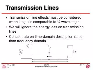
l l z Why Transmission Line? l Wavelength : propagation velocity l = frequency
In Free Space l At 10 KHz : = 30 km l At 10 GHz : = 3 cm Why Transmission Line? Transmission line behavior is prevalent when the structural dimensions of the circuits are comparable to the wavelength.
Justification for Transmission Line Let d be the largest dimension of a circuit circuit z l If d << l, a lumped model for the circuit can be used
Justification for Transmission Line circuit z l If d ≈ l, or d > l then use transmission line model
Modeling Interconnections Mid-range Frequency Low Frequency High Frequency or Short Transmission Line Lumped Reactive CKT
Wires in parallel near ground for d << D, h
Balanced, near ground for d << D, h
Coaxial Transmission Line TEM Mode of Propagation
Coaxial Air Lines Infinite Conductivity Finite Conductivity
Coaxial Connector Standards ConnectorFrequency Range 14 mm DC - 8.5 GHz GPC-7 DC - 18 GHz Type N DC - 18 GHz 3.5 mm DC - 33 GHz 2.92 mm DC - 40 GHz 2.4 mm DC - 50 GHz 1.85 mm DC - 65 GHz 1.0 mm DC - 110 GHz
Microstrip Characteristic Impedance 100 90 h = 21 mils 80 h = 14 mils h = 7 mils 70 Zo (ohms) 60 50 40 30 0 1 2 3 W/h Microstrip dielectric constant : 4.3.
Telegraphers’ Equations L: Inductance per unit length. C: Capacitance per unit length. Assume time-harmonic dependence
TL Solutions (Frequency Domain) forward wave backward wave
TL Solutions Propagation constant Propagation velocity Wavelength Characteristic impedance
Reflection Coefficient At z=0, we have V(0)=ZRI(0) But from the TL equations: Which gives where is the load reflection coefficient
Reflection Coefficient - If ZR = Zo, GR=0, no reflection, the line is matched - If ZR = 0, short circuit at the load, GR=-1 - If ZR inf, open circuit at the load, GR=+1 V and I can be written in terms of GR
Generalized Impedance Impedance transformation equation
Generalized Impedance - Short circuit ZR=0, line appears inductive for 0 < l < l/2 - Open circuit ZR inf, line appears capacitive for 0 < l < l/2 - If l = l/4, the line is a quarter-wave transformer
Generalized Reflection Coefficient Reflection coefficient transformation equation
Voltage Standing Wave Ratio (VSWR) We follow the magnitude of the voltage along the TL Maximum and minimum magnitudes given by
Voltage Standing Wave Ratio (VSWR) Define Voltage Standing Wave Ratio as: It is a measure of the interaction between forward and backward waves
VSWR – Arbitrary Load Shows variation of amplitude along line
VSWR – For Short Circuit Load Voltage minimum is reached at load
VSWR – For Open Circuit Load Voltage maximum is reached at load
VSWR – For Open Matched Load No variation in amplitude along line
Application: Slotted-Line Measurement • Measure VSWR = Vmax/Vmin • Measure location of first minimum
Application: Slotted-Line Measurement At minimum, Therefore, So, then Since and
Summary of TL Equations Voltage Current Impedance Transformation Reflection Coefficient Transformation Reflection Coefficient – to Impedance Impedance to Reflection Coefficient
Determining V+ For lossless TL, V and I are given by reflection coefficient at the load At z = -l,
Determining V+ this leads to or
Determining V+ Divide through by with and From which
TL Example • A signal generator having an internal resistance Zs = 25 W and an open circuit phasor voltage Vs = 1ej0 volt is connected to a 50-W lossless transmission line as shown in the above picture. The load impedance is ZR= 75 W and the line length is l/4. • Find the magnitude and phase of the load current IR.
Geometric Series Expansion Since V+ can be expanded in a geometric series form
TL Time-Domain Solution at z=0
TL Time-Domain Solution At z=-l
TL - Time-Domain Reflectometer For TDR, ZS = Zo GS = 0, and retain only k=1
Wave Shifting Method Forward traveling wave at port 1 (measured at near end of line) Forward traveling wave at port 2 (measured at far end of line) Backward traveling wave at port 1 (measured at near end of line) Backward traveling wave at port 2 (measured at far end of line)
Wave Shifting Solution* *Schutt-Aine & Mittra, Trans. Microwave Theory Tech., pp. 529-536, vol. 36 March 1988.
Frequency Dependence of Lumped Circuit Models • At higher frequencies, a lumped circuit model is no longer accurate for interconnects and one must use a distributed model • Transition frequency depends on the dimensions and relative magnitude of the interconnect parameters.