Download
1 / 26
280 likes | 723 Views
Stommel and Munk Theories of the Gulf Stream. October 8. Recall…. Integrate vertically:. Define Mass Transport Stream Function:. Now Sverdrup becomes:. WBC. Sverdrup Interior.

E N D
WBC Sverdrup Interior
Stommel (1948) and Munk (1949): Balance between vorticity input by wind, planetary vorticity, and frictional dissipation of vorticity in WBC, Leads to Closed Gyres: Parcels move S – f decreases, ω increases Parcels move N – f increases, ω decreases curl T < 0 → ω decreases so parcels must move S to compensate curl T > 0 → ω increases so parcels must move N to compensate WBC closes circulation and dissipates excess vorticity so parcels can rejoin interior
Figure 11.5 in Stewart. Stream function for flow in a basin as calculated by Stommel (1948). Left: Flow for non-rotating basin or flow for a basin with constant rotation. Right: Flow when rotation varies linearly with y.
Figure 11.6 in Stewart. Upper Left: Mean annual wind stress Tx(y) over the Pacific and the curl of the wind stress. Upper Right: The mass transport stream function for a rectangular basin calculated by Munk (1950) using observed wind stress for the Pacific. Lower Right: North-South component of the mass transport. From Munk (1950).
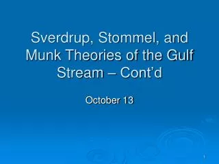
Figure 11.7 in Stewart. Sketch of the major surface currents in the North Atlantic. Values are transport in units of Sv=106 m3/s .
Figure 11.8 in Stewart. Detailed schematic of currents in the North Atlantic showing major surface currents. The numbers give the transport in units on 106 m3/s from the surface to a depth of 2000 m (?). Eg: East Greenland Current; Ei: East Iceland Current; Gu: Gulf Stream; Ir: Irminger Current; La: Labrador Current; Na: North Atlantic Current; Nc: North Cape Current; Ng: Norwegian Current; Ni: North Iceland Current; Po: Portugal Current; Sb: Spitsbergen Current; Wg: West Greenland Current. Numbers within squares give sinking water in units of 106m3/s. Solid Lines: Relatively warm currents. Broken Lines: Relatively cold currents.
Figure 11.9 in Stewart. Top Tracks of 110 drifting buoys deployed in the western North Atlantic. Bottom Mean velocity of currents in 2° × 2° boxes calculated from tracks above. Boxes with fewer than 40 observations were omitted. Length of arrow is proportional to speed. Maximum values are near 0.6 m/s in the Gulf Stream near 37°N 71°W.
Figure 11.10 in Stewart. Gulf Stream meanders lead to the formation of a spinning eddy, a ring. Notice that rings have a diameter of about 1°
Figure 11.11 in Stewart. Sketch of the position of the Gulf Stream, warm core, and cold core eddies observed in infrared images of the sea surface collected by the infrared radiometer on NOAA-5 in October and December 1978
Animations from Ocean Models • See http://www7320.nrlssc.navy.mil/global_nlom32/gfs.html • Click on 12 month mpegs for SSH, SST, and Currents
Let’s Review: Equations of Motion Linear momentum Continuity
Balance Between: Gives: A: 1 – 3 Inertial Oscillations B: 2 – 3 Geostrophy (frictionless) C: 2 – 3 – 5 Sverdrup (1947) (play tricks) D: 2 – 3 – 4 – 5 Munk (1950) solution (Stommel (1948) simplified eddy viscocity) B still applies in C and D – they were derived from B by looking at vorticity in addition to linear momentum Fundamental assumption in B, C, and D is “Steady” – no change with time
Ekman transport – Ekman Pumping – Vortex Stretching/Comperession
Sverdrup + Lateral drag/Eddy Viscocity = Stommel/Munk Gyres A A’