Download
1 / 46
470 likes | 624 Views
Dynamic connectivity algorithms for Feynman diagrams. Rubao Ji. Advisor: Dr. Robert W. Robinson Committee: Dr. E. Rodney Canfield Dr. Daniel M. Everett. 2002.11 . Outline of Thesis . Introduction

E N D
Dynamic connectivity algorithms for Feynman diagrams Rubao Ji Advisor: Dr. Robert W. Robinson Committee:Dr. E. Rodney Canfield Dr. Daniel M. Everett 2002.11
Outline of Thesis • Introduction • Algorithm design and time complexity analysis • Data structure and implementation • Experimental results and discussions
[ Introduction ] Feynman Diagram 5 A Feynman diagram with order of ncan be viewed as a matching on 2nnodes (edges in the matching are undirected and called V-lines) along with a permutation of the 2nnodes (represented by directed edges called G-lines) 3 2 4 0 1 G line V line
[ Introduction ] Feynman Diagram 2 A Feynman diagram with order of ncan be viewed as a matching on 2nnodes (edges in the matching are undirected and called V-lines) along with a permutation of the 2nnodes (represented by directed edges called G-lines) 3 5 4 1 0 G line V line
[ Introduction ] Feynman Diagram 2 A Feynman diagram with order of ncan be viewed as a matching on 2nnodes (edges in the matching are undirected and called V-lines) along with a permutation of the 2nnodes (represented by directed edges called G-lines) 5 3 4 1 0 G line V line
5 3 2 Switch(2,4) 4 5 0 3 2 1 5 4 0 3 2 1 Switch(4,0) 4 0 1 [ Introduction ] Switching and Connectivity a a´ Connected b b´ Switch(a,b) Not Connected a a´ b b´
2 5 3 4 1 0 [ Introduction ] Switching and Connectivity a a’ 5 b b’ 1 2 Switch(2,4) Switch(a,b) 0 3 4 a a’ b b’
[ Introduction ] Dynamic vs. Static • Dynamic graph problem: • Answer queries on graphs that are undergoing a sequence of updates (e.g. insertions and deletions of edges and vertices) • Fully-dynamic • Semi-dynamic (incremental, decremental) • Dynamic algorithm: • Update the solution of a problem more efficiently after dynamic changes rather than having to re-compute it from scratch each time (static).
[ Introduction ] Amortized & Expected • Running time of one single operation averaged over a • sufficiently long sequence of operations • Amortized Time • any sequence long enough • worst case bond • Expected Time • sequence has some distribution or is random • probabilistic worst case
[ Introduction ] A Brief History Deterministic algorithms Frederickson, 1985. O(m1/2) O(1) Epstein et al., 1992. O(n1/2) O(1) Henzinger&King, 1997. O(n1/3 log n) O(log n/loglog n) Holm et al., 1998. O(log2 n) O(log n/loglog n) Update Query Randomized algorithms Henzinger&King, 1995. O(log3 n) O(log n/loglog n) Henzinger&Thorup, 1997. O(log2 n) O(log n/loglog n) Thorup, 2000. O(log n(loglog n)3) O(log n/logloglog n) Update Query
[ Algorithm design and time complexity analysis ] Features that matter O (log n) O (log n) O (log? n) • Number of G-cycles • Update time • Query time
[ Algorithm design and time complexity analysis ] Lemma 2.1 For a randomly generated Feynman diagram of order n, the expected number of G-cycles is O(log n). Cl: G-cycle containing vertex v has length l v Prove: Pr [Cl]= 1/2n Pr [C1]= 1/2n Pr [C2]=(2n-1)/2n * 1/(2n-1) = 1/2n Pr [C3]=(2n-1)/2n * (2n-2)/(2n-1)*1/(2n-2) =1/2n :
[ Algorithm design and time complexity analysis ] Lemma 2.1 (cont’d) Xi : the size of the G-cycle containing node i S: total number of G-cycles
[ Algorithm design and time complexity analysis ] Update • Splay Tree (Self-Adjusting BST) • Treap (BST + Heap) G-cycle: In-order traversal V-line: Implicit numbering
[ Algorithm design and time complexity analysis ] Update • Splay Tree (Self-Adjusting BST) • Treap (BST + Heap) G-cycle: In-order traversal V-line: Implicit numbering
[ Algorithm design and time complexity analysis ] Update Lemma 2.2Each splay operation has an amortized time of O(log n) over (n) operations such that the tree size is always O(n). (From Sleator&Tarjan,1985) Lemma 2.3Each treap operation has an expected time of O(log n) averaged over all permutations of the nodes for the priority attribute. (From Seidel & Aragon, 1996)
[ Algorithm design and time complexity analysis ] Update: Splay Tree x Splay(x) x x t1 t2 t1 t2 Join(t1,t2) x x t1 t2 Split(x,t) x
[ Algorithm design and time complexity analysis ] Update: Treap delete(x) x Insert(x) x x t1 t2 t1 t2 delete(x) Join(t1,t2) b a Rotate left b a y t1 t2 Split(x,t) Rotate right x x x y
[ Algorithm design and time complexity analysis ] Query • SCQ (Simplified Connectivity Query) • ACQ (Advanced Connectivity Query) • IDQ (Integrated DFS Connectivity Query)
[ Algorithm design and time complexity analysis ] Query: SCQ • Straightforward approach • Simple DFS or pre-order traversal • Linear
[ Algorithm design and time complexity analysis ] Query: ACQ • More complicated than SCQ • Start from smallest component • O(log2 n)
[ Algorithm design and time complexity analysis ] Lemma 2.4 ACQ algorithm has an expected cost of O(log2n) time to query the connectivity of Feynman diagram. • Di The probability that, in examing vertices in the smallest component, a V -edge joining it to another component will be found in i attempts. D1> 1/2, D2> 1/2 + 1/4 … Dn> 1/2 + 1/4 + ··· +1/2(n-1) • SiThe probability that at least i attempts will be needed to find another component. Si> 1 - Di Ex[Steps] < 1 + 1/2 + 1/4 + …= 2 • O(log n) expected component, O(log n) expected joins, after each join, take O(log n) expected time to find the smallest component.
[ Algorithm design and time complexity analysis ] Query: IDQ • Integrated with update process • Maintain a G-cycle graph • O(log n)
[ Algorithm design and time complexity analysis ] IDQ (cont’d) Switch(a,b) a a b b Case 2 Case 1
[ Algorithm design and time complexity analysis ] IDQ (cont’d) Switch(a,b) a a b b Case 2 Case 1
[ Algorithm design and time complexity analysis ] IDQ (cont’d) Switch(a,b) a a b b Case 2 Case 1
[ Algorithm design and time complexity analysis ] IDQ (cont’d) IDQ algorithm has an expected cost of O(log n) time to query the connectivity of Feynman diagram. • DFS (Linear in number of G-cycles) • Chance of disconnected O(1/n) • If connected, O(1) to update the edge
[ Algorithm design and time complexity analysis ] Lemma 2.5 Using a splay forest data structure for Feynman diagram update combined with ACQ for connectivity queries gives an amortized expected time per operation of O(log2n). Using a treap forest data structure for Feynman diagram update combined with ACQ for connectivity queries gives an expected time per operation of O(log2n).
[ Algorithm design and time complexity analysis ] Lemma 2.6 Using a splay forest data structure for Feynman diagram update combined with IDQ for connectivity queries gives an amortized expected time per operation of O(log n). Using treap a forest data structure for Feynman diagram update combined with IDQ for connectivity queries gives an expected time per operation of O(log n).
[ Data structures and implementations ] Update -ASF ASF (Array-based Splay Forest) i lc[i] rc[i] p[i] s[i] 0 1 2 3 4 5 # # 0 # 2 # # # 5 # 1 3 ~2 4 ~4 5 4 2 1 1 4 1 6 2 4 2 1 0 5 3
[ Data structures and implementations ] ASF: Switch(a,b) { a T1, b T2} a b T1 Splay(a) Splay(b) T2 a´ b´ a b a´ b´ a´ b Switch a a b w b´ Splay(w) b´ a´ a´ w Switch (a,b) b b´ a Join w b a a´ b´ a´ b
[ Data structures and implementations ] ASF: Switch(a,b) {a ,b T} T T a´ a b b’ a a’ a´ b´ a b Splay(a) Splay(a) b b´ a a Switch (a,b) b´ b b’ a’ b a’ b b’ a Splay(b) a´ Splay(b) b b Reattach Reattach b’ a a’ b’ a b b b’ b’ a’ a’
[ Data structures and implementations ] Update -ATF ATF (Array-based Treap Forest) i lc[i] rc[i] p[i] s[i] prio[i] 0 1 2 3 4 5 # # 0 # 2 # # # 5 # 1 3 ~2 4 ~4 5 4 2 1 1 4 1 6 2 1 2 4 0 5 3 4 2 1 0 5 3
[ Data structures and implementations ] ATF: Switch(a,b) { a T1, b T2} Split(a) w w Split(b) T1 T2 a a’ b b’ a a’ b b’ Switch w w Delete(w) Delete(w) a b’ b a’ a b’ b a’ Join x Delete (x) a b’ b a’ a b’ b a’
[ Data structures and implementations ] ATF: Switch(a,b) {a ,b T} T T Split(a) Split(a) w b b’ a a’ a a’ b b’ w b b’ a a’ a a’ b b’ Split(b) Split(b) w w w w Reattach Reattach a’ b b’ b a’ b b’ a a’ b b’ b’ a a Delete(w) Delete(w) b a’ a b’
[ Data structures and implementations ] IDQ: Adjacency list 0 1 2 3 4 2 2 1 0 0 4 0 3 2 1 Type A node node visited down next 0 3 4 Type B node node visited p1 p2 adj_next link
[ Data structures and implementations ] IDQ: Switch(a,b) { a T1, b T2} 2 1 5 0 3 0 1 2 3 4 4 2 5 2 5 1 0 0 4 0 1 5 3 5 0 4
[ Data structures and implementations ] IDQ: Switch(a,b) {a ,b T} 0 1 2 3 4 0 1 5 6 3 4 2 2 1 0 0 2 5 2 6 1 1 0 0 4 0 4 0 3 3 6 2 1 1 5 0 3 0 3 4 4
[ Experimental results and discussion ] Exp 1: ASF vs. ATF • n: 10-100,000 • 5000 switches • ACQ • random
[ Experimental results and discussion ] Exp 2: Update vs. Query
[ Experimental results and discussion ] Exp 3: Frequency of Dis-connection
[ Experimental results and discussion ] Exp 4: Time per Switching
[ Experimental results and discussion ] Exp 5: IDQ/ACQ/SCQ
[ Experimental results and discussion ] Discussion • Splay tree vs. Treap • IDQ vs. ACQ vs. SCQ • Further study
Thanks ! Animation downloaded from: http://www.egglescliffe.org.uk/physics/particles/parts/parts1.html
[ Data structures and implementations ] ATF: Insert Insert(2) 0 Rotate(2) 2 Insert(5) 2 0 2 0 0 5 i W[i] P[i] 0 1 2 3 4 5 2 0 5 4 1 3 3 2 4 0 5 1 Insert(3) 2 Rotate(4) 2 Insert(4) 2 0 5 0 5 0 5 4 3 3 3 4 Rotate(4) 4 4 2 2 2 Rotate(4) Insert(1) 1 0 4 0 0 5 5 5 3 3 3