Download
1 / 12
130 likes | 747 Views
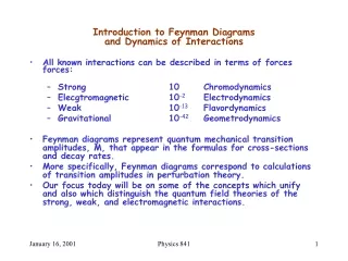
Introduction to Feynman Diagrams and Dynamics of Interactions. All known interactions can be described in terms of forces forces: Strong 10 Chromodynamics Elecgtromagnetic 10 -2 Electrodynamics Weak 10 -13 Flavordynamics Gravitational 10 -42 Geometrodynamics

E N D
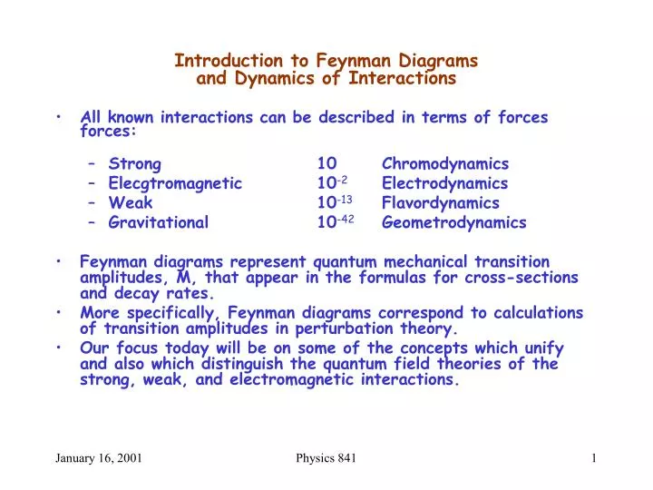
Introduction to Feynman Diagramsand Dynamics of Interactions • All known interactions can be described in terms of forces forces: • Strong 10 Chromodynamics • Elecgtromagnetic 10-2 Electrodynamics • Weak 10-13 Flavordynamics • Gravitational 10-42 Geometrodynamics • Feynman diagrams represent quantum mechanical transition amplitudes, M, that appear in the formulas for cross-sections and decay rates. • More specifically, Feynman diagrams correspond to calculations of transition amplitudes in perturbation theory. • Our focus today will be on some of the concepts which unify and also which distinguish the quantum field theories of the strong, weak, and electromagnetic interactions. Physics 841
time Quantum Electrodynamics (QED) • The basic vertex shows the coupling of a charged particle (an electron here) to a quantum of the electromagnetic field, the photon. Note that in my convention, time flows to the right. Energy and momentum are conserved at each vertex. Each vertex has a coupling strength characteristic of the interaction. • Moller scattering is the basic first-order perturbative term in electron-electron scattering. The invariant masses of internal lines (like the photon here) are defined by conservation of energy and momentum, not the nature of the particle. • Bhabha scattering is the process electron plus positron goes to electron plus positron. Note that the photon carries no electric charge; this is a neutral current interaction. Physics 841
Adding Amplitudes Note that an electron going backward in time is equivalent to an electron going forward in time. = M = + exchange annihilation Transition amplitudes (matrix elements) must be summed over indistinguishable initial and final states. Physics 841
More First Order QED • Essentially the same Feynman diagram describes the amplitudes for related processes, as indicated by these three examples. • The first amplitude describes electron positron annihilation producing two photons. • The second amplitude is the exact inverse, two photon production of an electron positron pair. • The third amplitude represents in the lowest order amplitude for Compton scattering in which a photon scatters from and electron producing a photon and an electron in the final state. Physics 841
Higher Order Contributions • Just as we have second order perturbation theory in non-relativistic quantum mechanics, we have second order perturbation theory in quantum field theories. • These matrix elements will be smaller than the first order QED matrix elements for the same process (same incident and final particles) because each vertex has a coupling strength . Physics 841
Putting it Together M = + + + + + Physics 841
Quantum Chromodynamics (QCD)[Strong Interactions] • The Feynman diagrams for strong interactions look very much like those for QED. • In place of photons, the quanta of the strong field are called gluons. • The coupling strength at each vertex depends on the momentum transfer (as is true in QED, but at a much reduced level). • Strong charge (whimsically called color) comes in three varieties, often called blue, red, and green. • Gluons carry strong charge. Each gluon carries a color and an anti-color. Physics 841
More QCD • Because gluons carry color charge, there are three-gluon and four-gluon vertices as well as quark-quark-gluon vertices. • QED lacks similar three-or four-photon vertices because the photon carries no electromagnetic charge. Physics 841
Vacuum Polarization -- in QED • Even in QED, the coupling strength is NOT a coupling constant. • The effective coupling strength depends on the effective dielectric constant of the vacuum:where is the effective dielectric constant. • Long distance low more dielectric (vacuum polarization) lower effective charge. (Simply an assertion here.) • Short distance higher effective charge. Physics 841
Vacuum Polarization -- in QCD • For every vacuum polarization Feynman diagram in QED, there is a corresponding vacuum polarization in QCD. • In addition, there are vacuum polarization diagrams in QCD which arise from gluon loops. • The quark loops lead to screening, as do the fermion loops in QED. The gluon loops lead to anti-screening. • The net result is that the strong coupling strength is large at long distance and small at short distance. Physics 841
Confinement in QCD • increases at small confinement. • As an example, is a color-singlet, . • Less obviously, is also a color-singlet, rgb. short distance hadronization time Physics 841
Weak Charged Current InteractionsA First Introduction • The quantum of the weak charged-current interaction is electrically charged. Hence, the flavor of the fermion must change. • As a first approximation, the families of flavors are distinct: • The coupling strength at each vertex is the same. Physics 841