Download
1 / 49
500 likes | 716 Views
Medical Image Analysis. Image Segmentation. Figures come from the textbook: Medical Image Analysis, by Atam P. Dhawan, IEEE Press, 2003. Edge-Based Image Segmentation. Useful links The Berkeley Segmentation Dataset and Benchmark TurtleSeg. Edge-Based Image Segmentation. Edge-based approach

E N D
Medical Image Analysis Image Segmentation Figures come from the textbook: Medical Image Analysis, by Atam P. Dhawan, IEEE Press, 2003.
Edge-Based Image Segmentation • Useful links • The Berkeley Segmentation Dataset and Benchmark • TurtleSeg
Edge-Based Image Segmentation • Edge-based approach • Spatial filtering to compute the first-order or second-order gradient information of the image: Sobel, Laplacian masks • Edges need to be linked to form closed regions • Uncertainties in the gradient information due to noise and artifacts in the image Figures come from the textbook: Medical Image Analysis, by Atam P. Dhawan, IEEE Press, 2003.
Edge Detection Operations • Gradient magnitude and directional information from the Sobel horizontal and vertical direction masks
Edge Detection Operations • The second-order gradient operator Laplacian can be computed by convolving one pf the following masks
Edge Detection Operations • A smoothing filter first before taking a Laplacian of the image • Combined into a single Laplacian of Gaussian function as
Edge Detection Operations • A Laplacian of Gaussian (LOG) mask of pixels, :
Boundary Tracking • Edge-linking • Pixel-by-pixel search to find connectivity among the edge segments • Connectivity can be defined using a similarity criterion among edge pixels • Geometrical proximity or topographical properties Figures come from the textbook: Medical Image Analysis, by Atam P. Dhawan, IEEE Press, 2003.
Boundary Tracking • The neighborhood search method • : edge magnitude • : edge orientation • : a boundary pixel • : a successor boundary pixel • , , :pre-determined thresholds
Boundary Tracking • A graph-based search method • Find paths between the start and end nodes minimizing a cost function that may be established based on the distance and transition probabilities • The start and end nodes are determined from scanning the edge pixels based on some heuristic criterion
Start Node End Node Figure 7.1. Top: An edge map with magnitude and direction information; Bottom: A graph derived from the edge map with a minimum cost path (darker arrows) between the start and end nodes.
Boundary Tracking • A* search algorithm • 1. Select an edge pixel as the start node of the boundary and put all of the successor boundary pixels in a list, OPEN • 2. If there is no node in the OPEN list, stop; otherwise continue • 3. For all nodes in the OPEN list, compute the cost function and select the node with the smallest cost . Remove the node from the OPEN list and label it as CLOSED. The cost function may be computed as
Boundary Tracking • A* search algorithm • 4. If is the end node, exit with the solution path by backtracking the pointers; otherwise continue • 5. Expand the node by finding all successors of . If there is no successor, go to Step 2; otherwise continue
Boundary Tracking • A* search algorithm • 6. If a successor is not labeled yet in any list, put it in the list OPEN with updated cost as and a pointer to its predecessor • 7. If a successor is already labeled as CLOSED or OPEN, update its value by • . Put those CLOSED successors whose cost functions were lowered, in the OPEN list and redirect to the pointers from all nodes whose costs were lowered. Go to Step 2
Hough Transform • Hough transform • Similar to the Radon transform • Detect straight lines and other parametric curves such as circles, ellipses • A line in the image space forms a point in the parameter space
Hough Transform Figure comes from the Wikipedia, www.wikipedia.org.
Gradiente O r p Figure 7.2. A model of the object shape to be detected in the image using Hough transform. The vector r connects the Centroid and a tangent point p. The magnitude and angle of the vector r are stored in the R-table at a location indexed by the gradient of the tangent point p. Figures come from the textbook: Medical Image Analysis, by Atam P. Dhawan, IEEE Press, 2003.
Pixel-Based Direct Classification Methods • Example the histogram for bimodal distribution • Find the deepest valley point between the two consecutive major peaks Figures come from the textbook: Medical Image Analysis, by Atam P. Dhawan, IEEE Press, 2003.
Figure 7.3. The original MR brain image (top), its gray-level histogram (middle) and the segmented image (bottom) using a gray value threshold T=12 at the first major valley point in the histogram.
Figure 7.3. The original MR brain image (top), its gray-level histogram (middle) and the segmented image (bottom) using a gray value threshold T=12 at the first major valley point in the histogram.
Figure 7.4. Two segmented MR brain images using a gray value threshold T=166 (top) and T=225 (bottom).
Optimal Global Thresholding • Assume • The histogram of an image to be segmented has two Gaussian distributions belonging to two respective classes such as background and object • The histogram
Optimal Global Thresholding • The error probabilities of misclassifying a pixel
Optimal Global Thresholding • Assume the Gaussian probability density functions
Optimal Global Thresholding • The optimal global threshold
Pixel Classification Through Clustering • Feature vector of pixels • Gray value, contrast, local texture measure, red, green, or blue components • Clusters in the multi-dimensional feature space • Group data points with similar feature vectors together in a single cluster • Distance measure: Euclidean or Mahalanobis distance • Post-processing • Region growing, pixel connectivity
K-Means Clustering • 1. Select the number of clusters with initial cluster centroids ; • 2. Partition the input data points into clusters by assigning each data point to the closest cluster centroid using the selected distance measure • 3. Compute a cluster assignment matrix representing the partition of the data points with the binary membership value of the th data point to the th cluster such that
K-Means Clustering • 4. Re-compute the centroids using the membership values as • 5. If cluster centroids or the assignment matrix does not change from the previous iteration, stop; otherwise go to Step 2.
K-Means Clustering • Objective function
Fuzzy c-Means Clustering • The objective function
Region-Based Segmentation • Region-growing based segmentation • Examine pixels in the neighborhood based on a pre-defined similarity criterion • The neighborhood pixels with similar properties are merged to form closed regions • Region splitting • The entire image or large regions are split into two or more regions based on a heterogeneity or dissimilarity criterion
Region-Growing • Two criteria • A similarity criterion that defines the basis for inclusion of pixels in the growth of the region • A stopping criterion that stops the growth of the region
Center Pixel Pixels satisfying the similarity criterion Pixels not satisfying the similarity criterion 3x3 neighborhood 5x5 neighborhood 7x7 neighborhood Segmented region Figure 7.5. A pixel map of an image (top) with the region-growing process (middle) and the segmented region (bottom).
Figure 7.6. A T-2 weighted MR brain image (top) and the segmented ventricles (bottom) using the region-growing method.
Region-Splitting • The following conditions are met: • 1. Each region, ; is connected • 2. • 3. for all , ; • 4. = TRUE for • 5. = FALSE for , where is a logical predicate for the homogeneity criterion on the region
R1 R21 R22 R24 R23 R41 R42 R3 R43 R44 R R4 R1 R2 R3 R44 R43 R41 R42 R24 R23 R21 R22 Figure 7.7. An image with quad region-splitting process (top) and the corresponding quad-tree structure (bottom).
Recent Advances in Segmentation • Model-based estimation methods • Rule-based systems • Automatic segmentation
Estimation-Model Based Adaptive Segmentation • A multi-level adaptive segmentation (MAS) method Figures come from the textbook: Medical Image Analysis, by Atam P. Dhawan, IEEE Press, 2003.
Define Classes Determination of Model Parameters (From a set of manually segmented and labeled images) Classification of Image Parameter Pixels Using Model Relaxation Signatures No No Yes Formation of All pixels a New Class classified? Necessary? Yes Identification of Tissue Classes and Pathology Figure 7.8: The overall approach of the MAS method.
Figure 7.9: (a) Proton Density MR and (b) perfusion image of a patient 48 hours after stroke.
Figure 7.10. Results of MAS method with 4x4 pixel probability cell size and 4 pixel wide averaging. (a) pixel classification as obtained on the basis of maximum probability, (b) as obtained with p>0.9.
Image Segmentation Using Neural Networks • Backpropagation neural network for classification • Radial basis function (RBF) network • Segmentation of arterial structure in digital subtraction angiograms Figures come from the textbook: Medical Image Analysis, by Atam P. Dhawan, IEEE Press, 2003.
x1 w1 x2 w2 wn Non-Linear Activation Function F wn+1 xn 1 Figure 7.11. A basic computational neural element or Perceptron for classification.
Output Layer Neurons Hidden Layer Neurons xn 1 x1 x2 x3 Figure 7.12. A feedforward Backpropagation neural network with one hidden layer.
Output Linear Combiner RBF Unit 2 RBF Unit 1 RBF Unit n RBF Layer Input Image Sliding Image Window Figure 7.13. An RBF network classifier for image segmentation.
Figure 7.14.RBF Segmentation of Angiogram Data of Pig-cast Phantom image (top left) with using a set of 10 clusters (top right) and 12 clusters (bottom) respectively.
Figure 7.14.RBF Segmentation of Angiogram Data of Pig-cast Phantom image (top left) with using a set of 10 clusters (top right) and 12 clusters (bottom) respectively.