Download
1 / 23
230 likes | 369 Views
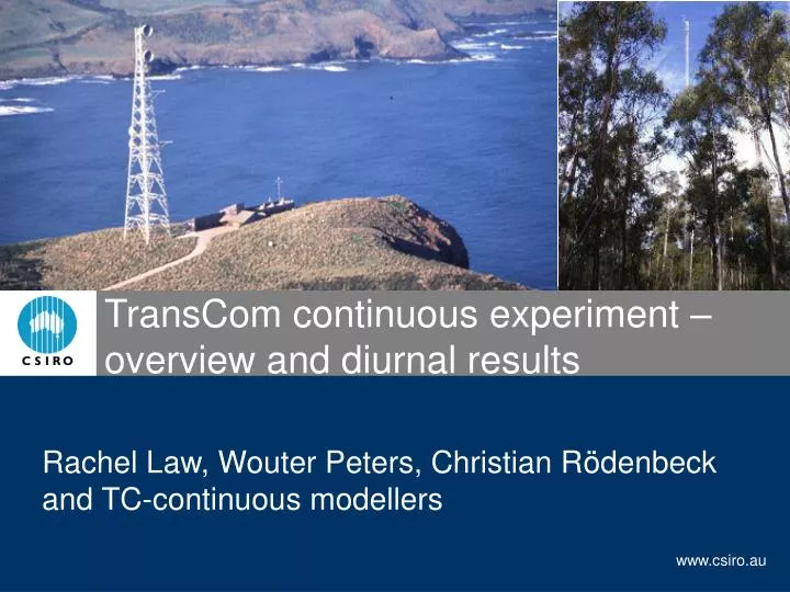
TransCom continuous experiment – overview and diurnal results. Rachel Law, Wouter Peters, Christian R ö denbeck and TC-continuous modellers. Outline – experiment overview. Background / Aim Fluxes Sites Models Output files General features of output. Background.

E N D
TransCom continuous experiment – overview and diurnal results Rachel Law, Wouter Peters, Christian Rödenbeck and TC-continuous modellers
Outline – experiment overview • Background / Aim • Fluxes • Sites • Models • Output files • General features of output
Background • Continuous CO2 contains flux information that is not captured in inversions using monthly mean data Cape Grim, Australia Pallas, Finland
Fluxes • SiB biosphere fluxes • Hourly • Daily • Monthly • CASA biosphere fluxes • 3 hourly • Monthly • Fossil - 1998 • 4. Ocean (Takahashi-02) • 5. SF6 • 6. Radon
Sites – ‘allsite.list’ • 280 locations: modellers chose how to sample e.g. nearest grid-point or interpolate. Land and ocean point requested for coastal sites
Sites – ‘contsite.list’ • 100 locations: • Tracer concentration output for all model levels to 500 hPa • Met variables: u, v, pressure for all levels to 500 hPa • Trace gas flux, surface pressure, cloud cover, boundary layer height
Output files • Submitted files for 2002 and 2003 (models run from 2000) • all.MODEL.INSTITUTION.yyyy.nc – contains trace gas concentration for 9 tracers at 280 sites. Also latitude, longitude, level, land arrays • tracer.MODEL.INSTITUTION.yyyy.nc – one file for each tracer, all levels to 500 hPa, 100 sites. Also tracer flux. • met.MODEL.INSTITUTION.yyyy.nc – met data • Processed files • SITE.MODEL.INSTITUTION.yyyy.nc – all the data for a single site for each model. Currently for 50 sites.
Things to watch out for … • Check where model has sampled: lat, lon, land/ocean • Check level – in ‘all’ file some models always sampled surface layer, most chose levels above the surface for sites with altitude > ~100m • Profile information useful because removes altitude choice • Flux information very useful – confirms whether models sampling similar conditions • Some models were unable to submit all the data: IFS – 3 hourly output; DEHM – subset of tracers COMET – only ‘all’ files • Many models have been revised since their original submission to fix bugs or add missing data
Outline – diurnal results • Observations • Model data processing • Summer diurnal cycle • Case studies • Vertical resolution • Seasonal cycle of diurnal amplitude • Conclusions and paper
Data processing • 3 tracers : CASA (3hr), Taka02, fossil98 • Fit with trend and harmonics: Cfit = a1 + a2t + a3cos(2πt)+a4sin(2πt)+a5cos(4πt)+a6sin(4πt) • Residuals: Cresid = C – Cfit • Sum residuals : CASA+Taka02+fossil98 • For each month, average residuals by hour of day to give mean diurnal cycle • Average June, July, August; calculate amplitude as max concentration – min concentration • NB daily diurnal amplitude calculated at fixed time of day (may be <= max-min conc for that day)
Summer diurnal amplitude (JJA) • Black cross – models • Red dot – observations • Sites plotted by continent and latitude • Large range – models span observed • Sampling location contributes e.g. high altitude sites Asia Europe America
Case studies: 1. Mikawa-Ichinomiya Mean summer diurnal cycle Black, obs; colours, models • Colour and line style indicate flux magnitude • Zero (blue), small (cyan), moderate (green), large (red) biosphere flux • Small (solid), large (dash) fossil flux
Which level represents high altitude sites? Obs Obs Mt Cimone: LMDZ level 2-7 Plateau Rosa: TM5_eur, level 3-8
Amplitude vs phase Mt Cimone, CMN, 2165m Plateau Rosa, PRS, 3480m Zugspitze/Schneefernerhaus, ZGP, 2960m Sonnblick, SNB, 3106m
Flux towers: Tapajos, Brazil Mean diurnal CO2 concentration, JJA Mean CO2 flux, JJA
Distribution of diurnal amplitude (JJA) Tapajos, Brazil Boreas, Canada
Synoptic variation in amplitude: Boreas Jul 24 Aug 18
Is model vertical resolution important? Concentration to flux ratio at 7 surface sites Ptp diurnal amplitude concentration divided by CASA flux amplitude plus fossil flux Most models give similar ratio Small influence from vertical resolution Some variation across sites e.g. TPJ vs FRD
Seasonal cycle of diurnal amplitude Fraserdale Mace Head Tapajos Neuglobsow Amplitude normalised by mean amplitude across 12 months
Conclusions • Valuable dataset for comparing modelled CO2 with in-situ records • To realistically sample most sites, probably need better than 2x2o resolution • Moderate to high altitude sites remain a challenge • For the diurnal cycle most models show similar strengths and weaknesses compared to observations • Seasonal and synoptic changes in diurnal amplitude show some model skill • More detailed analysis required before observed diurnal cycle of CO2 routinely used in inversions
Overview paper 1 • Diurnal cycle only • Probable target journal: Global Biogeochemical Cycles • Almost complete, sec 5.1.2 is possible addition • Revised DEHM to be included, LMDZ fluxes now available • Submission by end of May?