Download
1 / 91
910 likes | 924 Views
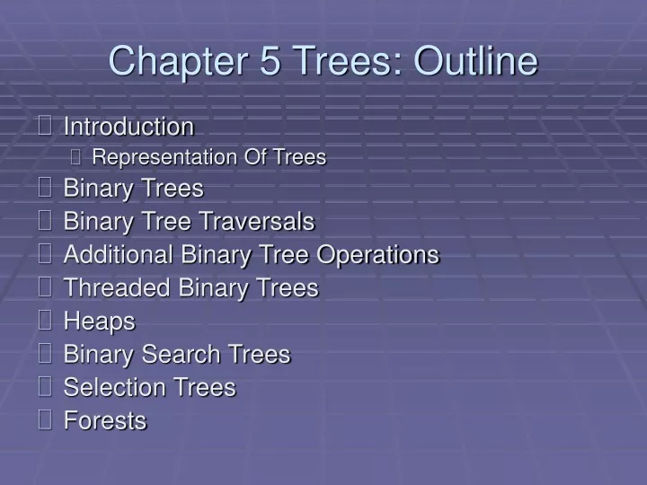
Chapter 5 Trees: Outline. Introduction Representation Of Trees Binary Trees Binary Tree Traversals Additional Binary Tree Operations Threaded Binary Trees Heaps Binary Search Trees Selection Trees Forests. Introduction (1/8).

E N D
Chapter 5 Trees: Outline • Introduction • Representation Of Trees • Binary Trees • Binary Tree Traversals • Additional Binary Tree Operations • Threaded Binary Trees • Heaps • Binary Search Trees • Selection Trees • Forests
Introduction (1/8) • A tree structure means that the data are organized so that items of information are related by branches • Examples:
Introduction (2/8) • Definition (recursively): A tree is a finite set of one or more nodes such that • There is a specially designated node called root. • The remaining nodes are partitioned into n>=0 disjoint set T1,…,Tn, where each of these sets is a tree. T1,…,Tn are called the subtrees of the root. • Every node in the tree is the root of some subtree
Introduction (3/8) • Some Terminology • node: the item of information plus the branches to each node. • degree: the number of subtrees of a node • degree of a tree: the maximum of the degree of the nodes in the tree. • terminal nodes (or leaf): nodes that have degree zero • nonterminal nodes: nodes that don’t belong to terminal nodes. • children: the roots of the subtrees of a node X are the children of X • parent: X is the parent of its children.
Introduction (4/8) • Some Terminology (cont’d) • siblings:children of the same parent are said to be siblings. • Ancestors of a node: all the nodes along the path from the root to that node. • The level of a node: defined by letting the root be at level one. If a node is at level l, then it children are at level l+1. • Height (or depth): the maximum level of any node in the tree
Level A 1 B C 2 H 3 D E F G I 4 Introduction (5/8) Property:(# edges) = (#nodes) - 1 • Example Ais the rootnode B is theparent of D and E C is thesibling of B D and E are thechildren of B D, E, F, G, I areexternal nodes, orleaves A, B, C, Hare internal nodes The level of Eis 3 The height (depth) of the tree is4 The degree of nodeBis 2 The degree of the treeis3 Theancestors of nodeIis A, C, H The descendants of nodeCisF, G, H, I
Introduction (6/8) • Representation Of Trees • List Representation • we can write of Figure 5.2 as a list in which each of the subtrees is also a list ( A ( B ( E ( K, L ), F ), C ( G ), D ( H ( M ), I, J ) ) ) • The root comes first, followed by a list of sub-trees
Introduction (7/8) • Representation Of Trees (cont’d) • Left Child-Right Sibling Representation
Introduction (8/8) • Representation Of Trees (cont’d) • Representation As A Degree Two Tree
A A B B Binary Trees (1/9) • Binary trees are characterized by the fact that any node can have at most two branches • Definition (recursive): • A binary tree is a finite set of nodes that is either empty or consists of a root and two disjoint binary trees called the left subtree and the right subtree • Thus the left subtree and the right subtree are distinguished • Any tree can be transformed into binary tree • by left child-right sibling representation
Binary Trees (2/9) • The abstract data type of binary tree
Binary Trees (3/9) • Two special kinds of binary trees: (a) skewed tree, (b) complete binary tree • The all leaf nodes of these trees are on two adjacent levels
Binary Trees (4/9) • Properties of binary trees • Lemma 5.1 [Maximum number of nodes]: • The maximum number of nodes on level i of a binary tree is 2i-1, i1. • The maximum number of nodes in a binary tree of depth k is 2k-1, k1. • Lemma 5.2 [Relation between number of leaf nodes and degree-2 nodes]: For any nonempty binary tree, T, if n0 is the number of leaf nodes and n2 is the number of nodes of degree 2, then n0 = n2 + 1. • These lemmas allow us to define full and complete binary trees
Binary Trees (5/9) • Definition: • A full binary tree of depth k is a binary tree of death k having 2k-1 nodes, k 0. • A binary tree with n nodes and depth k is complete iff its nodes correspond to the nodes numbered from 1 to n in the full binary tree of depth k. • From Lemma 5.1, the height of a complete binary tree with n nodes is log2(n+1)
A 1 [1] [2] [3] [4] [5] [6] [7] A B C — D — E B C 2 3 Level 1 Level 2 Level 3 D E 4 5 6 7 Binary Trees (6/9) • Binary tree representations (using array) • Lemma 5.3: If a complete binary tree with n nodes is represented sequentially, then for any node with index i, 1 i n, we have • parent(i) is at i /2 if i 1. If i = 1, i is at the root and has no parent. • LeftChild(i) is at 2iif 2i n. If 2i n, then i has no left child. • RightChild(i) is at 2i+1 if 2i+1 n. If 2i +1 n, then i has no left child
Binary Trees (7/9) • Binary tree representations (using array) • Waste spaces: in the worst case, a skewed tree of depth k requires 2k-1 spaces. Of these, only k spaces will be occupied • Insertion or deletion of nodes from the middle of a tree requires the movement of potentially many nodesto reflect the change in the level of these nodes
Binary Trees (8/9) • Binary tree representations (using link)
Binary Trees (9/9) • Binary tree representations (using link)
V : visiting node L: moving left R: moving right right_child data left_child Binary Tree Traversals (1/9) • How to traverse a tree or visit each node in the tree exactly once? • There are six possible combinations of traversal LVR, LRV, VLR, VRL, RVL, RLV • Adopt convention that we traverse left before right, only 3 traversals remain LVR (inorder), LRV (postorder), VLR (preorder)
Binary Tree Traversals (2/9) • Arithmetic Expression using binary tree • inorder traversal (infix expression) A / B * C * D + E • preorder traversal (prefix expression) + * * / A B C D E • postorder traversal (postfix expression) A B / C * D * E + • level order traversal + * E * D / C A B
Binary Tree Traversals (3/9) • Inorder traversal (LVR) (recursive version) output: A / B * C * D + E ptr L V R
Binary Tree Traversals (4/9) • Preorder traversal (VLR) (recursive version) output: + * * / A B C D E V L R
Binary Tree Traversals (5/9) • Postorder traversal (LRV) (recursive version) output: A B / C * D * E + L R V
14 11 17 E D C 3 4 5 8 1 2 A * * / + B Binary Tree Traversals (6/9) • Iterative inorder traversal • we use a stack to simulate recursion L V R output: A / B * C * D + E node
Binary Tree Traversals (7/9) • Analysis of inorder2 (Non-recursive Inorder traversal) • Let n be the number of nodes in the tree • Time complexity: O(n) • Every node of the tree is placed on and removed from the stack exactly once • Space complexity: O(n) • equal to the depth of the tree which (skewed tree is the worst case)
Binary Tree Traversals (8/9) • Level-order traversal • method: • We visit the root first, then the root’s left child, followed by the root’s right child. • We continue in this manner, visiting the nodes at each new level from the leftmost node to the rightmost nodes • This traversal requires a queue to implement
17 11 14 C E D 4 8 5 1 2 3 * * A / B + Binary Tree Traversals (9/9) • Level-order traversal (using queue) output: + * E * D / C A B FIFO ptr
Additional Binary Tree Operations (1/7) • Copying Binary Trees • we can modify the postorder traversal algorithm only slightly to copy the binary tree similar as Program 5.3
Additional Binary Tree Operations (2/7) • Testing Equality • Binary trees are equivalent if they have the same topology and the information in corresponding nodes is identical V L R the same topology and data as Program 5.6
Additional Binary Tree Operations (3/7) • Variables: x1, x2, …, xn can hold only of two possible values, true or false • Operators: (and), (or), ¬(not) • Propositional Calculus Expression • A variable is an expression • If x and y are expressions, then ¬x, xy, xy are expressions • Parentheses can be used to alter the normal order of evaluation (¬> >) • Example: x1 (x2 ¬x3)
Additional Binary Tree Operations (4/7) • Satisfiability problem: • Is there an assignment to make an expression true? • Solution for the Example x1 (x2 ¬x3) : • If x1 and x3 are false and x2 is true • false (true ¬false) = false true = true • For n value of an expression, there are 2n possible combinations of true and false
data X3 value X3 X1 X2 X1 Additional Binary Tree Operations (5/7) (x1 ¬x2)(¬ x1 x3)¬x3 postorder traversal
Additional Binary Tree Operations (6/7) • node structure • For the purpose of our evaluation algorithm, we assume each node has four fields: • We define this node structure in C as:
T F T T F Additional Binary Tree Operations (7/7) • Satisfiability function • To evaluate the tree is easily obtained by modifying the original recursive postorder traversal L R V node TRUE TRUE FALSE FALSE TRUE TRUE FALSE FALSE TRUE TRUE FALSE TRUE
Threaded Binary Trees (1/10) • Threads • Do you find any drawback of the above tree? • Too many null pointers in current representation of binary trees n: number of nodes number of non-null links: n-1 total links: 2n null links: 2n-(n-1) = n+1 • Solution: replace these null pointers with some useful “threads”
Threaded Binary Trees (2/10) • Rules for constructing the threads • If ptr->left_child is null, replace it with a pointer to the node that would be visited beforeptrin aninorder traversal • If ptr->right_child is null, replace it with a pointer to the node that would be visited afterptrin aninorder traversal
A C f t t f B E G F D inorder traversal: I H H D I B E A F C G Threaded Binary Trees (3/10) • A Threaded Binary Tree root t: true thread f: false child dangling dangling
Threaded Binary Trees (4/10) • Two additional fields of the node structure, left-thread and right-thread • If ptr->left-thread=TRUE, then ptr->left-child contains a thread; • Otherwise it contains a pointer to the left child. • Similarly for the right-thread
Threaded Binary Trees (5/10) • If we don’t want the left pointer of H and the right pointer of G to be dangling pointers, we may create root node and assign them pointing to the root node
Threaded Binary Trees (6/10) • Inorder traversal of a threaded binary tree • By using of threads we can perform an inorder traversal without making use of a stack (simplifying the task) • Now, we can follow the thread of any node, ptr, to the “next” node of inorder traversal • If ptr->right_thread = TRUE, the inorder successor of ptr is ptr->right_child by definition of the threads • Otherwise we obtain the inorder successor of ptr by following a path of left-child links from the right-child of ptr until we reach a node with left_thread = TRUE
Threaded Binary Trees (7/10) • Finding the inorder successor (next node) of a node threaded_pointer insucc(threaded_pointer tree){ threaded_pointer temp; temp = tree->right_child; if (!tree->right_thread) while (!temp->left_thread) temp = temp->left_child; return temp; } tree temp Inorder
Threaded Binary Trees (8/10) • Inorder traversal of a threaded binary tree void tinorder(threaded_pointer tree){ /* traverse the threaded binary tree inorder */ threaded_pointer temp = tree; for (;;) { temp = insucc(temp); if (temp==tree) break; printf(“%3c”,temp->data); } } output: H D I B E A F C G tree Time Complexity: O(n)
Threaded Binary Trees (9/10) • Inserting A Node Into A Threaded Binary Tree • Insert childas the right child of node parent • change parent->right_thread to FALSE • set child->left_thread and child->right_thread to TRUE • set child->left_child to point to parent • set child->right_child to parent->right_child • change parent->right_child to point to child
X X Threaded Binary Trees (10/10) • Right insertion in a threaded binary tree void insert_right(thread_pointer parent, threaded_pointer child){ /* insert child as the right child of parent in a threaded binary tree */ threaded_pointer temp; child->right_child = parent->right_child; child->right_thread = parent->right_thread; child->left_child = parent; child->left_thread = TRUE; parent->right_child = child; parent->right_thread = FALSE; If(!child->right_thread){ temp = insucc(child); temp->left_child = child; } } root parent A B C child temp parent A child B C D Second Case First Case E F successor
Heaps (1/6) • The heap abstract data type • Definition: A max(min) tree is a tree in which the key value in each node is no smaller (larger) than the key values in its children. Amax(min) heap is a complete binary tree that is also amax(min) tree • Basic Operations: • creation of an empty heap • insertion of a new elemrnt into a heap • deletion of the largest element from the heap
Heaps (2/6) • The examples of max heaps and min heaps • Property: The root ofmax heap(min heap)containsthelargest(smallest) element
Heaps (3/6) • Abstract data type of Max Heap
Heaps (4/6) • Queue in Chapter 3: FIFO • Priority queues • Heaps are frequently used to implement priority queues • delete the element with highest (lowest) priority • insert the element with arbitrary priority • Heaps is the only way to implement priority queue machine service: amount of time (min heap) amount of payment (max heap) factory: time tag
Heaps (5/6) • Insertion Into A Max Heap • Analysis of insert_max_heap • The complexity of the insertion function is O(log2n) insert 21 5 *n= 6 5 i= 3 3 7 6 1 [1] 20 21 parent sink [2] [3] item upheap 15 20 2 5 [5] [6] [7] [4] 10 14 2 5
< Heaps (6/6) • Deletion from a max heap • After deletion, the heap is still a complete binary tree • Analysis of delete_max_heap • The complexity of the insertion function is O(log2n) parent = 2 1 4 *n= 4 5 child = 4 2 8 [1] 15 20 [2] [3] 14 15 2 item.key = 20 [4] [5] temp.key = 10 10 14 10