Download

1 / 59
710 likes | 1.2k Views
Tries. Multiway Trees. Trees with possibly more than two branches at each node are know as Multiway trees. 1. Orchards, Trees, and Binary Trees 2. Lexicographic Search Trees: Tries 3. External Searching: B-Trees 4. Red-Black Trees. Lexicographic Search Trees: Tries.

E N D
Multiway Trees Trees with possibly more than two branches at each node are know as Multiway trees. 1. Orchards, Trees, and Binary Trees 2. Lexicographic Search Trees: Tries 3. External Searching: B-Trees 4. Red-Black Trees
Lexicographic Search Trees: Tries • We can apply the idea of table lookup to information retrieval from a tree by using a key or part of a key to make a multiway branch. • Instead of searching by comparison of entire keys, we can consider a key as a sequence of characters, and use these characters to determine a multiway branch at each step. • We make a 26-way branch according to the first letter of the name, followed by another branch according to the second letter, and so on. • This multiway branching is the idea of a thumb index in a dictionary.
Lexicographic Search Trees: Tries • A thumb index is generally used only to find the words with a given initial letter; some other search method is then used to continue. • In a computer we can proceed two or three levels by multiway branching, but then the tree will become too large, and we shall need to resort to some other device to continue.
Lexicographic Search Trees: Tries • To keep the size of such a multiway tree we could prune all the branches from the tree that do not lead to any key. • e.g., in English, there are no words that begin with the letters ‘bb’, ‘bc’, ‘bf’, ‘bg’ …, but there are words beginning with ‘ba’, ‘bd’, or ‘be’. • Hence all the branches and nodes for nonexixtent words can be removed from the tree. • The resulting tree is called a trie. • This term originated as letters extracted from the word retrieval.
Lexicographic Search Trees: Tries DEFINITION: - A trie of order mis either empty or consists of an ordered sequence of exactly m tries of order m.
Searching for a Key in Tries • A trie describing the English words (as listed in the Oxford English Dictionary) made up only from the letters a, b, and c is shown in Figure 11.7. • Along with the branches to the next level of the trie, each node contains a pointer to a record of information about the key, if any, that has been found when the node is reached. • The search for a particular key begins at the root. The first letter of the key is used as an index to determine which branch to take. • An empty branch means that the key being sought is not in the tree. • Otherwise, we use the second letter of the key to determine the branch at the next level, and so continue.
Searching for a Key in Tries • When we reach the end of the word, the information pointer directs us to the desired information. • We shall use a NULLinformation pointer to show that the string is not a word in the trie. • Note, therefore, that the word a is a prefix of the word aba, which is a prefix of the word abaca. • On the other hand, the string abac is not an English word, and therefore its node has a NULL information pointer.
Lexicographic Search Trees: Tries • The number of steps required to search a trie or insert into it is proportional to the number of characters making up a key, not to a logarithm of the number of keys as in other tree-based searches. No. of searces No. of characters in the key.
Insertion into a Trie • Adding a new key to a trie is quite similar to searching for the key: • We must trace our way down the trie to the appropriate point and set the data pointer to the information record for the new key. • If, on the way, we hit a NULL branch in the trie, we must not terminate the search, but instead we must create new nodes and put them into the trie so as to complete the path corresponding to the new key.
Deletion from a Trie • The same general plan used for searching and insertion also works for deletion from a trie. • We trace down the path corresponding to the key being deleted, and when we reach the appropriate node, we set the corresponding data member to NULL. • If now, however, this node has all its members NULL(all branches and the data member), then we should delete this node. • To do so, we can set up a stack of pointers to the nodes on the path from the root to the last node reached. • Alternatively, we can use recursion in the deletion algorithm and avoid the need for an explicit stack.
Assessment of Tries • The number of steps required to search a trie (or insert into it) is proportional to the number of characters making up a key, not to a logarithm of the number of keys as in other tree-based searches. • If this number of characters is small relative to the (base 2) logarithm of the number of keys, then a trie may prove superior to a binary tree. • If, for example, the keys consist of all possible sequences of five letters, then the trie can locate any of n = 265 = 11,881,376 keys in 5 iterations, whereas the best that binary search can do is lg n 23.5 key comparisons.
Assessment of Tries • In many applications, however, the number of characters in a key is larger, and the set of keys that actually occur is sparse in the set of all possible keys. • In these applications, the number of iterations required to search a trie may very well exceed the number of key comparisons needed for a binary search. • The best solution, finally, may be to combine the methods. A trie can be used for the first few characters of the key, and then another method can be employed for the remainder of the key. • If we return to the example of the thumb index in a dictionary, we see that, in fact, we use a multiway branch to locate the first letter of the word, but we then use some other search method to locate the desired word among those with the same first letter.
External Searching • So far we have assumed that all our data structures are kept in high-speed memory; that is, we have considered only internal information retrieval. • For many applications, this assumption is reasonable, but for many other important applications, it is not. • Let us now turn briefly to the problem of external information retrieval, where we wish to locate and retrieve records stored in a file.
Access Time • The time required to access and retrieve a word from high-speed memory is a few nanoseconds at most. • The time required to locate a particular record on a disk is measured in milliseconds, and for floppy disks can exceed a second. • Hence the time required for a single access is millions of times greater for external retrieval than for internal retrieval. block of storage: • On the other hand, when a record is located on a disk, the normal practice is not to read only one word, but to read in a large page or block of information at once, to save time. • Typical sizes for blocks range from 256 to 1024 characters or words.
Access Time • Why should it matter? • speed of access: • memory: 10 nsec typical (10/1,000,000,000 seconds) • disk: milliseconds (1/1000 seconds) • floppy disk: seconds • A normal binary search in 1000 elements would access memory for log21000 = 10 x 10 ns where as 10 harddisk access would be 1000000x10 ns.
Access Time • Our goal in external searching must be to minimize the number of disk accesses, since each access takes so long compared to internal computation. • With each access, however, we obtain a block that may have room for several records. • Using these records we may be able to make a multiway decision concerning which block to access next. • Hence multiway trees are especially appropriate for external searching.
Multiway Search Trees • Binary search trees generalize directly to multiway (m-way) search trees in which, for some integer m called the orderof the tree, each node has at mostm children. • If k m is the number of children, then the node contains exactly k - 1 keys, which partition all the keys in the subtrees into k subsets. • If some of these subsets are empty, then the corresponding children in the tree are empty. • Figure 11.8 shows a 5-way search tree (between 1 and 4 entries in each node) in which some of the children of some nodes are empty.
A 5-way search tree (not a B-tree) • since some nodes have empty children, some have too few children, and the leaves are not all on the same level.
Multiway Search Trees • An m-way search tree is a tree in which, for some integer m called the order of the tree, each node has at most m children. • If k m is the number of children, then the node contains exactly k - 1 keys, which partition all the keys into k subsets.
Multiway Search Tree • We want a “Multiway Search Tree” that minimizes file accesse. • Each node should be a block of data on the disk: • Each node then requires a read of the disk, and each link points to a logical “area” of the disk file
minimize disk reads • Movement level to level requires another disk read. • so, we want the number of levels to be few. i.e. the height of the tree should be as small as possible. • We want to minimize disk reads
Searches are costly • we want all searches to terminate in the same number of accesses • i.e. don’t want long searches and short searches, rather balanced performance • so insist that all leaves are at the same level.
minimal number of children • Insist that every node have some minimal number of children • this helps us get “the most” from each node
Access Time • don’t want: prefer:
B-Tree • A B-Tree is a special type of multiway search tree that satisfies the design goals discussed above. • As we look at the definition of a B-Tree we will notice that the design goals outlined above are incorporated directly into the definition. • We will discuss this definition and look at some examples of structures that are and are not B-Trees.
Balanced Multiway Trees • Our goal is to devise a multiway search tree that will minimize file accesses; hence we wish to make the height of the tree as small as possible. • We can accomplish this by insisting, • first, that no empty subtrees appear above the leaves (so that the division of keys into subsets is as efficient as possible); • second, that all leaves be on the same level (so that searches will all be guaranteed to terminate with about the same number of accesses); and, • third, that every node (except the leaves) have at least some minimal number of children. We shall require that each node (except the leaves) have at least half as many children as the maximum possible. • These conditions lead to the following formal definition:
A B-Tree of order 2 • A B-Tree of order 2 is a complete binary search tree. • These all honour rules 1 & 2, but violate rule 3 • adding rule 3, these are all B-trees of order 2
Insertion into a B-Tree In contrast to binary search trees, B-trees are not allowed to grow at their leaves; instead, they are forced to grow at the root. General insertion method: 1. Search the tree for the new key. This search (if the key is truly new) will terminate in failure at a leaf. 2. Insert the new key into to the leaf node. If the node was not previously full, then the insertion is finished. 3. When a key is added to a full node, then the node splits into two nodes, side by side on the same level, except that the median key is not put into either of the two new nodes. 4. When a node splits, move up one level, insert the median key into this parent node, and repeat the splitting process if necessary. 5. When a key is added to a full root, then the root splits in two and the median key sent upward becomes a new root. This is the only time when the B-tree grows in height.
The quick brown fox jumpes over the lazy dog. A B-tree of order 5 will contain up to 4 keys in each node.
Deletion from a B-Tree • If the entry that is to be deleted is not in a leaf, then its immediate predecessor (or successor) under the natural order of keys is guaranteed to be in a leaf. • We promote the immediate predecessor (or successor) into the position occupied by the deleted entry, and delete the entry from the leaf. • If the leaf contains more than the minimum number of entries, then one of them can be deleted with no further action. • If the leaf contains the minimum number, then we first look at the two leaves (or, in the case of a node on the outside, one leaf) that are immediately adjacent to each other and are children of the same node. If one of these has more than the minimum number of entries, then one of them can be moved into the parent node, and the entry from the parent moved into the leaf where the deletion is occurring. • If the adjacent leaf has only the minimum number of entries, then the two leaves and the median entry from the parent can all be combined as one new leaf, which will contain no more than the maximum number of entries allowed. • If this step leaves the parent node with too few entries, then the process propagates upward. In the limiting case, the last entry is removed from the root, and then the height of the tree decreases.
Red-Black Tree • In your text book, the writer has used a contiguous list to store the entries within a single node of a B-tree. • Doing so was appropriate because the number of entries in one node is usually relatively small and because we were emulating methods that might be used in external files on a disk, where dynamic memory may not be available, and records may be stored contiguously on the disk.
Red-Black Tree • In general, however, we may use any ordered structure we wish for storing the entries in each B-tree node. • Small binary search trees turn out to be an excellentchoice. • We need only be careful to distinguish between the links within a single B-tree node and the links from one B-tree node to another. • Let us therefore draw the links within one B-tree node as curly colored lines and the links between B-tree nodes as straight black lines. • Figure 11.16 shows a B-tree of order 4 constructed this way.