Download
1 / 18
190 likes | 562 Views
Topics: Multiple Regression Analysis (MRA). Review Simple Regression Analysis Multiple Regression Analysis Design requirements Multiple regression model R 2 Testing R 2 and b’s Comparing models Comparing standardized regression coefficients. Multiple Regression Analysis (MRA).

E N D
Topics: Multiple Regression Analysis (MRA) • Review Simple Regression Analysis • Multiple Regression Analysis • Design requirements • Multiple regression model • R2 • Testing R2 and b’s • Comparing models • Comparing standardized regression coefficients
Multiple Regression Analysis (MRA) • Method for studying the relationship between a dependent variable and two or more independent variables. • Purposes: • Prediction • Explanation • Theory building
Design Requirements • One dependent variable (criterion) • Two or more independent variables (predictor variables). • Sample size: >= 50 (at least 10 times as many cases as independent variables)
Assumptions • Independence: the scores of any particular subject are independent of the scores of all other subjects • Normality: in the population, the scores on the dependent variable are normally distributed for each of the possible combinations of the level of the X variables; each of the variables is normally distributed • Homoscedasticity: in the population, the variances of the dependent variable for each of the possible combinations of the levels of the X variables are equal. • Linearity: In the population, the relation between the dependent variable and the independent variable is linear when all the other independent variables are held constant.
One dependent variable Y predicted from one independent variable X One regression coefficient r2: proportion of variation in dependent variable Y predictable from X One dependent variable Y predicted from a set of independent variables (X1, X2 ….Xk) One regression coefficient for each independent variable R2: proportion of variation in dependent variable Y predictable by set of independent variables (X’s) Simple vs. Multiple Regression
Example: The Model • Y’ = a + b1X1 + b2X2 + …bkXk • The b’s are called partial regression coefficients • Our example-Predicting AA: • Y’= 36.83 + (3.52)XASC + (-.44)XGSC • Predicted AA for person with GSC of 4 and ASC of 6 • Y’= 36.83 + (3.52)(6) + (-.44)(4) = 56.23
Multiple Correlation Coefficient (R) and Coefficient of Multiple Determination (R2) • R = the magnitude of the relationship between the dependent variable and the best linear combination of the predictor variables • R2 = the proportion of variation in Y accounted for by the set of independent variables (X’s).
Explaining Variation: How much? Predictable variation by the combination of independent variables Total Variation in Y Unpredictable Variation
Proportion of Predictable and Unpredictable Variation (1-R2)= Unpredictable (unexplained) variation in Y Where: Y= AA X1 = ASC X2 =GSC Y X1 R2 = Predictable (explained) variation in Y X2
Various Significance Tests • Testing R2 • Test R2 through an F test • Test of competing models (difference between R2) through an F test of difference of R2s • Testing b • Test of each partial regression coefficient (b) by t-tests • Comparison of partial regression coefficients with each other - t-test of difference between standardized partial regression coefficients ()
Example: Testing R2 • What proportion of variation in AA can be predicted from GSC and ASC? • Compute R2: R2 = .16 (R = .41) : 16% of the variance in AA can be accounted for by the composite of GSC and ASC • Is R2 statistically significant from 0? • F test: Fobserved = 9.52, Fcrit (05/2,100) = 3.09 • Reject H0: in the population there is a significant relationship between AA and the linear composite of GSC and ASC
Example: Comparing Models -Testing R2 • Comparing models • Model 1: Y’= 35.37 + (3.38)XASC • Model 2: Y’= 36.83 + (3.52)XASC + (-.44)XGSC • Compute R2 for each model • Model 1: R2 = r2 = .160 • Model 2: R2 = .161 • Test difference between R2s • Fobs = .119, Fcrit(.05/1,100) = 3.94 • Conclude that GSC does not add significantly to ASC in predicting AA
Testing Significance of b’s • H0: = 0 • tobserved = b - standard error of b • with N-k-1 df
Example: t-test of b • tobserved = -.44 - 0/14.24 • tobserved = -.03 • tcritical(.05,2,100) = 1.97 • Decision: Cannot reject the null hypothesis. • Conclusion: The population for GSC is not significantly different from 0
Comparing Partial Regression Coefficients • Which is the stronger predictor? Comparing bGSC and bASC • Convert to standardized partial regression coefficients (beta weights, ’s) • GSC = -.038 • ASC = .417 • On same scale so can compare: ASC is stronger predictor than GSC • Beta weights (’s ) can also be tested for significance with t tests.
Different Ways of Building Regression Models • Simultaneous: all independent variables entered together • Stepwise: independent variables entered according to some order • By size or correlation with dependent variable • In order of significance • Hierarchical: independent variables entered in stages
Practice: • Grades reflect academic achievement, but also student’s efforts, improvement, participation, etc. Thus hypothesize that best predictor of grades might be academic achievement and general self concept. Once AA and GSC have been used to predict grades, academic self-concept (ASC) is not expected to improve the prediction of grades (I.e. not expected to account for any additional variation in grades)