Download
1 / 36
360 likes | 496 Views
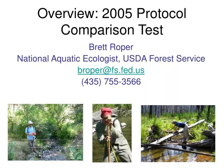
Overview: 2005 Protocol Comparison Test. Brett Roper National Aquatic Ecologist, USDA Forest Service broper@fs.fed.us (435) 755-3566. Analysis. To determine stream means and difference among streams proc mixed data=***; classes stream ; model BW = stream;

E N D
Overview: 2005 Protocol Comparison Test Brett Roper National Aquatic Ecologist, USDA Forest Service broper@fs.fed.us (435) 755-3566
Analysis To determine stream means and difference among streams procmixed data=***; classes stream ; model BW = stream; lsmeans stream /pdiff adjust=tukey; ods output diffs=ppp lsmeans=mmm; ods listing exclude diffs lsmeans; run; %include 'c:\BBRfile\stats\sasmacros\pdmix800.sas'; %pdmix800(ppp,mmm,alpha=0.1,sort=yes); run; No analysis yet to determine significant differences among groups For Means, STD, CV procglm data= ***; class stream; model BW = stream; run; To decompose variance procmixed data=***; classes stream; model BW =; random stream; run;
Proc GLM statement Source DF Squares Mean Square F Value Pr > F Model 11 254.5044526 23.1367684 148.70 <.0001 Error 24 3.7342700 0.1555946 Corrected Total 35 258.2387225 R-Square Coeff Var Root MSE grad Mean 0.985539 10.57097 0.394455 3.731490 Proc Mixed statement Covariance Parameter Estimates Cov Parm Estimate Stream 7.6604 Residual 0.1556
Output of the PDMIX statement for gradient from one group Standard Letter Obs Stream Estimate Error Group 1 Myrtle 9.8156 0.2277 A 2 Whisky 7.1933 0.2277 B 3 Indian 6.0044 0.2277 C 4 Crawfish 5.2956 0.2277 C 5 WF Lick 3.5644 0.2277 D 6 Tinker 2.9444 0.2277 DE 7 Potamus 2.7622 0.2277 DE 8 Trail 1.9511 0.2277 EF 9 Big 1.3800 0.2277 F 10 Crane 1.3756 0.2277 F 11 Camus 1.3601 0.2277 F 12 Bridge 1.1311 0.2277 F
Group 1 = Group 2 - 5 What should the results of an aquatic habitat protocol comparison look like?
What is a good attribute • For categorization • Very little Rosgen large classes • For status and trend • Minimum • S:N of around 2, % stream ≈ 70% (I would prefer S:N of 4 and stream ≈ 80% • Coefficient of variation ≈ 20%
Attributes • Gradient • Bankfull Width • Wetted Width • Width-to-Depth • Sinuosity • Entrenchment • % Pool • Residual Pool Depth • %Fines • Median Particle Size • D84 • Large Wood • Large wood volume
Myrtle Crane
Correlations among all stream width groups and the truth (remember these are mean values compared to the truth) truth GRP 1 GRP 2 GRP 3 GRP 4 GRP 5 GRP 6 truth 1.00 0.97 0.96 0.89 0.96 0.97 0.97 Group 1 1.00 0.99 0.90 0.97 0.96 0.97 Group 2 1.00 0.93 0.98 0.97 0.98 Group 3 1.00 0.89 0.95 0.95 Group 4 1.00 0.93 0.96 Group 5 1.00 0.99 Group 6 1.00
Width to Depth Big Crawfish
Entrenchment Big Crawfish
Lets look at Percent Pool Crane Myrtle
How I summarized • A: S:N >9, stream variability 90%, CV < 20% • B: S:N >4, stream variability 80%, CV < 20% • C: S:N > 2, Stream variability 70% or CV around 20% • D: S:N close to 2, stream variability more than 50%, or CV around 20%. • F: Anything lower.
Preliminary Observations • Some attributes everyone does passable at: gradient, bankfull width, wetted width, residual pool depth. • For these attributes it is likely that cross walks can be determined not only with e ach other but with the truth. • Only one attribute that nobody does well at; entrenchment. • Although nobody does well with this one it may not matter since it will only be used for classification; but if that is true why not as a group agree on an AML. • For remaining attributes – width to depth, sinousity, % pool, D50D84, fines, bank stability, and large wood volume – some groups have better (more consistent within the group) protocols than others.
Some thoughts on why certain attributes were done better when there was variation in the protocols • Ratio things (Sinuosity, width-to-depth, and entrenchment) were done better with laser level. • Extensive training resulted in more consistent sediment (fines and particle distributions, and large wood (counts and volume). • Pools were best done with a fixed length.
How do we decide what to measure Bankfull width vs wetted width • Bankfull width has hydrologic meaning, can be measured if the stream is dry. Not affect by season. • Wetted with more consistently measured, is a measure of summer aquatic habitat (nice to know a stream is dry)
What’s next? • LiDAR • Determine what steps should be taken to standardize protocols. • Continue efforts to develop crosswalks. • Should data quality control recommendations be made. • Seek consensus on the best protocol(s) to use. • Determine which attributes provide useful data. • Proposal was submitted for BPA funding for follow up work. • Publication of the John Day basin protocol test results.