Download
1 / 29
290 likes | 412 Views
Pacific Northwest Side-by-Side Aquatic Habitat Protocol Comparison Test. Steve Lanigan, Brett Roper, John Buffington, Eric Archer, Scott Downie, Phil Kaufmann, Shannon Hubler, Kim Jones, Glenn Merritt, Deborah Konnoff, Allen Pleus, Michael Ward, Keith Wolf, John Faustini, Russ Faux. AREMP.

E N D
Pacific Northwest Side-by-Side Aquatic Habitat Protocol Comparison Test Steve Lanigan, Brett Roper,John Buffington, Eric Archer, Scott Downie, Phil Kaufmann, Shannon Hubler, Kim Jones, Glenn Merritt, Deborah Konnoff, Allen Pleus, Michael Ward, Keith Wolf, John Faustini, Russ Faux
AREMP Watershed Sciences This comparison was a group effort (PNAMP) UCB $$ =
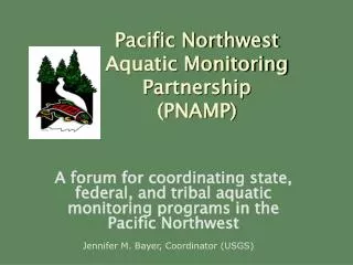
Pacific Northwest Aquatic Monitoring Partnership Protocol Comparison Monitoring Group
Project Objectives • Evaluate aquatic habitat protocols to determine which are the “best” at minimizing among crew variation while maximizing differences among streams. • Determine if relationships can be developed among different protocols for the same attribute. • Do these results reflect some true value?
John Day Basin July-Aug, 2005 • Eight agency and tribal field monitoring groups independently evaluated 12 reaches with multiple (generally 3) crews. • One intensive monitoring group (“truth”, 3 to 9 days per site) • LiDAR flights (coarse “truth”)
Overview of study design & “truth” protocol Wadable streams: 1-15 m width, slope; 0-10% • 3 channel types • Plane-bed (Tinker, Bridge, Camas, Potamus) • Pool-riffle (WF Lick, Crane, Trail, Big) • Step-pool (Whiskey, Myrtle, Indian, Crawfish) plane-bed pool-riffle step-pool
Many attributes were evaluated; the results depend on the attribute • %Fines • D84 • Large Wood • Entrenchment • Median Particle Size • Gradient • Bankfull Width • Width-to-Depth • % Pool • Residual Pool Depth • Sinuosity
Group 1 = Group 2 - 5 Objectives 1 & 2; What should the data looklike if attributes are consistently measured within a group and comparable among groups?
Bankfull Width A A A C C B A Exceeds Within Groups Quality Control Standard Meets Within Groups Quality Control Standard
Can results be shared with each other? Bankfull width (m)
Bankfull Width to Depth D F C F F B Exceeds within groups quality control standard Meets within groups quality control standard Doesn’t meet within groups quality control standard
Can results be shared with each other? Bankfull width to depth
You want the truth? You can’t handle the truth!
How was truth defined? Crane Ck (reach length = 80 channel widths) contour interval = 10 cm riffle bar survey points pool
But even “truth” is sensitive to methodology • Example: average bankfull width at Trail Ck, derived from “truth” data set • 8.48 m = average of 5 equally spaced cross sections • 8.79m = average of all 75 cross sections • 7.81 m = total bankfull volume of the channel divided by total bankfull surface area, both determined from a topographic map constructed from all total station data
How comparable are field data to more precisely defined truth?
Field data vs Remotely Sensed Channel Morphology (e.g., LiDAR)? • Channel morphology parameters can be generated from topographic layers derived from the LiDAR data: • stream centerline • wetted width • bankfull width • Topographic indictors include: 1) visible terraces, 2) slope/ gradient inflections, 3) contours. • Digital multi-spectral imagery provide additional indictors including: 1) permanent vegetation, 2) bar extents • floodprone width • valley bottom
Trail Creek Hillshade of ½ meter scale bare earth Digital Elevation Model True color image draped over ½ meter vegetation model
Comparison of LiDAR derived cross sections to Group 3 ground level data: Trail Creek Site #1
Comparison of LiDAR derived cross sections to Group 3 ground level data: Trail Creek Site #3
Preliminary Findings - The good news! • There is wide-spread interest in: • Improving stream habitat data quality. • Sharing data among state, tribal, and federal monitoring programs. • Making protocols comparable through standardization and/or developing statistical relationships among different programs.
Preliminary Findings - The good news! • There are a number of stream attributes that can be used to indicate the status and trend of a aquatic system in a cost efficient manner. • Based on preliminary work, there seems to be a strong relationship between rapid field measurements and more intensive field efforts.
Where more work can help… • Quality control - Some attributes are not consistently measured within a monitoring group. • Some group’s protocols for attributes (though definition and/or training) are better than others: Should there be minimum standards for protocols?, How should they be set? • Because protocols definitions do differ among groups, more effort is needed to insure these data can be shared. • Understanding the relationship between a monitoring groups answer for an attribute and “truth.”