Download
1 / 11
110 likes | 269 Views
Gridding and preconditioning in ASKAPsoft. Max Voronkov, Tim Cornwell ASKAP Computing 24 th August 2010. Convolutional gridding: basics. Measurements don’t lie on a regular grid Convolve with some function Sample the result of this convolution at regular grid points.

E N D
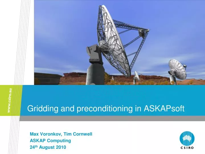
Gridding and preconditioning in ASKAPsoft Max Voronkov, Tim Cornwell ASKAP Computing 24th August 2010
Convolutional gridding: basics • Measurements don’t lie on a regular grid • Convolve with some function • Sample the result of this convolution at regular grid points need gridding to be able to use FFT Size of the convolution kernel C(∆u,∆v) affects the performance • Kernel C(∆u,∆v) is calculated at a finer grid (oversampling) • Appropriate oversampling plane is chosen on the basis of u and v • Grid correction: divide the image by FT of the kernel • One of the simplest kernels - prolate spheroidal function • Optimal aliasing reduction, very compact (7x7 pixels in ASKAPsoft) • Oversampling factor is hard coded to be 128 in ASKAPsoft
Convolutional gridding: AProject and WProject • Convolution done during gridding comes out as a multiplication at the image domain • Normally we do grid correction to remove this effect (i.e divide by FT of the kernel) • However, one can apply image plane multiplicative effects by choosing a CF appropriately (and not grid-correcting for it) Phase screen in the image plane defined by the w-term primary beam (mosaicing) and w-term can both be taken into account via special choice of convolution functions FT of this gives CF of the w-projection algorithm This term of the mosaicing equation can be calculated via CF. This is A-projection algorithm
WProject gridder: convolution functions Phase screen for a large w-term Phase screen for a small w-term • Single offset beam • Frame = w-plane • CF is FT of • Size depends on the w-term! CSIRO
AWProject gridder: convolution functions Phase screen = phase gradient locally = offset in the uv domain • Simulated single offset beam • Each frame = single w-plane Size depends on the w-term Offset depends on the w-term
Support of convolution function (CF) CFs are generated in a maxsupport x maxsupport buffer Support is searched using a given threshold (cutoff parameter) We throw an exception if found support exceeds the ratio image size / oversample Then we extract oversample2 slices, support x support each (oversample is a stride factor in slicing of the CF) Example of the convolution function for a large w-term (single oversampling plane) CSIRO
WStack and AProjectWStack gridders ww1 ww2 wwN ……………….. Stacking algorithms need more memory than projection algorithms, but usually require less computations (convolution functions have smaller support) Stack of grids w-term can be accounted for in the image domain Each visibility is gridded into the most appropriate grid from the stack according to its w-term The final image is a sum across FTs of all grids, each multiplied by the image plane w-term
Preconditioning = weighting (in the uv-domain) Noise power can be defined via robustness: • Traditional weighting schemes require two gridding passes • First pass to form visibility weight • Second pass to grid the product of visibilities and appropriate weights • In ASKAPsoft we apply linear filters to images • One iteration over visibility data is sufficient • We use term ‘preconditioning’ because this filtering serves to regularise a system of normal equations which is solved at the minor cycle • Another interpretation is to improve PSF to make deconvolution easier • Two main preconditioning options have been implemented: • Gaussian tapering • Wiener filter (somewhat related to Robust weighting)
Wiener filter, tapering: PSFs 10’’ taper, filter with R=-1 No taper, no filter No taper, filter with R=-1 Emil Lenc developed a nice tool to visualize ASKAP PSF for different sets of parameters (note, images are not final; still work in progress): http://www.atnf.csiro.au/people/Emil.Lenc/ASKAP/psf/sim/view.html http://www.atnf.csiro.au/people/Emil.Lenc/ASKAP/psf/dingo/view.html
Summary • ASKAPsoft has a number of gridder options implemented • Variable and offset CF support makes the imaging much faster! • Offset support is really needed for mosaicing gridders only • Support search procedure is parameterized by cutoff. Lower cutoff means larger support, slower execution but higher accuracy. • ASKAPsoft can handle the w-term via either the projection or stacking • Stacking is usually faster, but requires more memory • Both algorithms allow parallelization on w-term • Memory bandwidth considerations may favour the stacking algorithm (each grid is independent during gridding) • Traditional weighting schemes (e.g. Robust or uniform weighting) require two iterations over visibility data • ASKAPsoft uses preconditioning (filtering) instead • A combination of Wiener filter and tapering gives nice results CP Applications / Calibration and Imaging
Contact Us Phone: 1300 363 400 or +61 3 9545 2176 Email: enquiries@csiro.au Web: www.csiro.au Thank you Australia Telescope National Facility Max Voronkov Software Scientist (ASKAP) Phone: 02 9372 4427 Email: maxim.voronkov@csiro.au Web: http://www.atnf.csiro.au/projects/askap/ CP Applications / Calibration and Imaging