Download
1 / 20
200 likes | 324 Views
Advanced Preconditioning for Generalized Least Squares. Recall: To stabilize the inversions, we minimize the objective function J where. where m is the damping or regularization parameter.

E N D
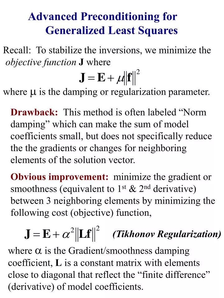
Advanced Preconditioning for Generalized Least Squares Recall: To stabilize the inversions, we minimize the objective function J where where m is the damping or regularization parameter. Drawback: This method is often labeled “Norm damping” which can make the sum of model coefficients small, but does not specifically reduce the the gradients or changes for neighboring elements of the solution vector. Obvious improvement: minimize the gradient or smoothness (equivalent to 1st & 2nd derivative) between 3 neighboring elements by minimizing the following cost (objective) function, (Tikhonov Regularization) where a is the Gradient/smoothness damping coefficient, L is a constant matrix with elements close to diagonal that reflect the “finite difference” (derivative) of model coefficients.
Calculation of L matrix (a matrix that acts on model vector and returns a vector containing second derivatives of model coefficients) To find elements to this matrix, let’s start with 1st derivative of a function f (1) Newton Forward A crude way to estimate the derivative at a pointxi is by a forward difference operator (h is x spacing): (2) Newton Backward estimate the derivative at a pointxi by a backward difference operator: (3) Realizing that the derivative approximations above are really derivatives at (i+h/2) and (i-h/2), we can rewrite
This is what is often called “1st-order finite difference” form, where h is the x-spacing or index spacing, depending on application (it is assumed constant), so if h=1 (index change from one to another element of filter), using Forward Newton we have Note: This is not a square matrix! By minimizing first derivative with model coef f, But after doing LTL, it becomes a square matrix with the same dimension as CTC
Now, the second derivative can be estimated from these two first-order ones at index (i), if h=1 (index change from one to another element of filter), we have So the L matrix for smoothness (2nd derivative of model parameter) can be computed as follows
Resolution of an Inverse Problem Resolution of a given inverse problem is about how well a given model (assume we know already, even though we don’t for most problems) can be recovered by the inversion procedure (with the damping ---- norm, gradient, or smoothness constraints). Two ways to assess model resolution for Generalized Least Squares (example below is for normal damping): 1. Through analysis of Resolution Matrix 2. Through simulated inversion procedure of known model predictions. Resolution Matrix: Suppose then
Now, of course, to get stable solutions to inverse problem we regularize and seek: If things work well, we are hoping that the following approximate relationship holds (R is resolution Matrix): Reality: If there is damping, R is not the identify matrix. Even if there is no damping, finding the inverse is only a least-squares estimate and therefore the above is Not true! That said, R gives us a way to assess how close we are in finding the exact solution. Key here: We must have a way of obtaining that q matrix, which is often not given by various inversion procedures. SVD comes to rescue!
2nd way to assess resolution: Checkerboard Tests • Basic Procedure: • Make the solution vector look like a known, simple pattern (‘checkerboards’ are used in testing the Earth’s structure in 2D or 3D, while square-wave looking signals (on and off) are used for 1D problems) • Using this known, hypothetical solution to make predictions of data. Assume these computed values as parts of the data vector (right-hand side). In other words, for any A X = B problem, assume X’ to have the following pattern 3D 1D 2D Then make predictions B’ based on this geometrical solution.
Continued: Checkerboard Test Procedures • One can use B’ as the data vector, or add some random noise to B’ to simulate imperfect data (where the level of noise should reflect that of the real data vector) • Solve the problem AX’’=B’ where A is the same as before (with all sorts of operations like norm & roughness regularizations). For fairness, make sure it is same procedure and matrix as you would find the real solution (which, does not look like checkerboard, one that we hope to assess the accuracy and resolution). Find X’’. • The similarity (amplitude, phase) between X’ (input checkerboard) and X’’ (recovered checkerboard under all conditions of the real data inversion) provides an effective measure of the resolution the inversion problem using the damping/regularization (or Sing. Value removal) that you used for the real data.
Resolution Test Surface wave velocity structure of Alberta: Shen & Gu, 2012 • Idea: • Introduce a spherical harmonic pattern • shoot rays through that model (must be same rays as the real data set), get a set of fake observations • Based on the ray geometries and this hypothetical data set, invert for the structure back. See if the recovered checkerbord agrees with input model. 9 Issue: This is the minimum requirement, not a sufficient one. An inversion procedure that does not produce a good checkerboard has no merit, but one that does still may or may not be correct.
Hypothesis Test Based on the tomographic map of the final model, generate a simple representation of it, then try to recover this simple representation with the same inversion/damping criterion and the same data set. In principle, this is not too different from checkerboard test. Advantage over checkerboard: more relevant scales and sizes of the anomaly to resolve. Sometime used in combination with standard checkerboard. Atlas &Eaton (2006), on structure beneath Great Lakes Standard Checkerboard Test
Another example of hypothesis testing Rawlinson et al., 2010
Jackknifing/Bootstrap Test Throw in randomly selected subsets of the data, recover a model and compare with one that uses the entire data set. The consistency is a good indication of the data & method resolution. To a great extent, the models produced by various researchers of the same structure could be considered an in-situ test as they represents results from different subsets of the data (with overlaps) and infer similar but also different structures. The stability of the results (without considerations of modeling strategies) are indication of resolution. Rawlinson et al., 2010
Alternative Solution: Monte-Carlo Method and Genetic Algorithms: Random walk but with probalistic models. A more probable solution (say a solution that decreases error) would have a greater chance of survival for the next step. To speed up the solution, can use derivatives of the models and residuals as a guide. But nothing is absolute, so that one won’t easily get trapped into a local minimum. An example of finding area of a region by randomly shooting darts to dartboard Radomness These are forward approaches to solving an inverse problem. The Monte-Carlo approach is somewhat “blind” in finding a final solution that produce a goodness of fit. GA is more scientific using the law of “natural selection” to find models with better “genes” in an iterative way.
Another Example of Monte Carlo: Observed seismogram (top) near Italy. The bottom traces are results of Monte-Carlo fit (by varying the seismic structure randomly within certain limits at depths). In a strict sense, the Monte-Carlo approach is really forward fitting rather than inversions!! Okeler, Gu et al., 2009, GJI.
Resulting seismic (shear velocity) structure with depth. Some “training” must be done to impose reasonable bounds to the randomly varying seismic speeds. Statistics will help quantifying the amount of variations and obtain the “average” structure.
Nonlinear Problems Solutions: (1) use Monte-carlo to explore the answer (2) use Iterative procedures to linearize Earthquake Location Inversion (highly nonlinear) Station i (xi, yi, 0) Epicenter Earthquake Focus (x, y, z) m=(m1, m2, m3, m4) = (T, x, y, z) Suppose station i detects an earthquake at arrival time d’i which depends on origin time t0 and travel time between source and station T(x, xi) d’i = t0+ T(x, xi)
Forward approach: (1) make an educated guess where this earthquake may have occurred based on travel time curve (2) Assume an earth structure model, compute predicted travel time di_pred= Fi(m) (3) Compute residual between actual and predicted time: ri=d’i - Fi(m) (4) Grid search for m such that tolerance < SUM |ri| (L1 norm) or tolerance < SUM (ri)2 (L2 norm) Inversion approach: (1) Again, assume a good “educated” guess of location and time, get a model m0 (2) Setup the problem m = m0 + D m
In order to minimize residuals, we seek Dm such that Now, this becomes a linear AX = b problem. In other words, through iterations, we have obtained a linear problem involving PERTURBATIONS of model parameters.