Download
1 / 21
550 likes | 1.38k Views
REGRESI LINIER SEDERHANA (SIMPLE LINEAR REGRESSION). Matakuliah : KodeJ0204/Statistik Ekonomi Tahun : Tahun 2007 Versi : Revisi. REGRESI LINIER SEDERHANA (SIMPLE LINEAR REGRESSION). CAKUPAN MATERI: Model Regresi Linier Sederhana Metode Kuadrat Terkecil (Least Squares Method)

E N D
REGRESI LINIER SEDERHANA (SIMPLE LINEAR REGRESSION) Matakuliah : KodeJ0204/Statistik Ekonomi Tahun : Tahun 2007 Versi : Revisi
REGRESI LINIER SEDERHANA (SIMPLE LINEAR REGRESSION) CAKUPAN MATERI: • Model Regresi Linier Sederhana • Metode Kuadrat Terkecil (Least Squares Method) • Koefisien Determinasi • Asumsi Model • Uji Keberartian (Testing for Significance) • Estimasi dengan Persamaan Regresi • Analisis Residual: Pemeriksaan Asumsi Model
REGRESI LINIER SEDERHANA (SIMPLE LINEAR REGRESSION) • Model Regresi Linier Sederhana y = 0 + 1x+ • Persamaan Regresi Linier Sederhana E(y) = 0 + 1x • Estimasi Persamaan Regresi Linier Sederhana y = b0 + b1x dimana y = variabel tak bebas (response/dependent variable) x = variabel bebas (predictor/independent variable) = suku sisaan (error/residual) 0 = intercept (titik potong garis regresi dengan sumbu y) 1 = slope/kemiringan garis regresi ^
METODE KUADRAT TERKECIL • Kriteria Kuadrat Terkecil Prinsip: Meminimalkan jumlah kuadrat jarak/selisih antara nilai variabel tak bebas sebenarnya dengan nilai estimasi variabel tak bebas (error) dimana: yi = nilai observasi ke-i dari variable tak bebas yi = nilai estimasi ke-i dari variabel tak bebas ^
METODE KUADRAT TERKECIL • Kemiringan (Slope) Persamaan Regresi Estimasi • Intercept Persamaan Regresi Estimasi dimana: xi = nilai variabel bebas untuk observasi ke-i yi = nilai variabel tak bebas untuk observasi ke-i x = rata-rata nilai variabel bebas y = rata-rata nilai variabel tak bebas n = total observasi
CONTOH: REED AUTO SALES Sebagai bagian dari kampanyenya, Reed Auto menggunakan media televisi untuk iklan selama akhir pekan yang lalu. Berikut adalah data dari 5 sampel penjualan. Banyaknya iklan TVJumlah Mobil Terjual 1 14 3 24 2 18 1 17 3 27
CONTOH: REED AUTO SALES • Kemiringan Persamaan Regresi Estimasi b1 = 220 - (10)(100)/5 = 5 24 - (10)2/5 • Intercept Persamaan Regresi Estimasi b0 = 20 - 5(2) = 10 • Estimasi Persamaan Regresi y = 10 + 5x Interpretasi: Jika banyaknya iklan bertambah 1 kali, maka dapat meningkatkan banyak penjualan mobil sebanyak 5. ^
CONTOH: REED AUTO SALES • Scatter Diagram 30 25 20 y = 5x + 10 15 Jumlah Mobil Terjual 10 5 0 0 1 2 3 4 Banyaknya Iklan TV
KOEFISIEN DETERMINASI • Hubungan antara SST, SSR, SSE SST = SSR + SSE • Koefisien Determinasi (Coefficient of Determination) r2 = SSR/SST dimana: SST = total sum of squares SSR = regression sum of squares SSE = error sum of squares
KOEFISIEN KORELASI SAMPEL dimana: b1 = slope persamaan regresi estimasi
CONTOH: REED AUTO SALES • KOEFISIEN DETERMINASI r2 = SSR/SST = 100/114 = 0,8772 Artinya: Hubungan regresi sangat kuat karena 88% variasi mobil yang terjual dapat dijelaskan oleh banyaknya iklan TV. • KOEFISIEN KORELASI
ASUMSI MODEL • Asumsi tentang suku sisaan (error), • Error merupakan suatu random variabel dengan rata-rata nol (E()=0). • Varian error , dinotasikan dengan 2, adalah sama untuk semua nilai variabel bebas (homoscedastic). • Nilai saling bebas (non autocorrelation). • Sisaan terdistribusi normal.
UJI SIGNIFIKANSI • Untuk menguji keberartian hubungan regresi, maka harus dilakukan uji hipotesis apakah b1 sama dg nol. • Dua pengujian yang umum digunakan adalah Uji t dan Uji F • Kedua pengujian di atas memerlukan estimasi varian dari dalam model regresi, s2. • Mean square error (MSE) menghasilkan estimasi untuk varian . s2 = MSE = SSE/(n-2) dimana:
UJI SIGNIFIKANSI: Uji t • Hipotesis H0: 1 = 0 Ha: 1 0 • Statistik Uji dimana • Aturan Penolakan Tolak H0 jika t < -t/2 atau t > t /2 dimana t/2 didasarkan pada distribusi t dengan derajat bebas n - 2.
CONTOH: REED AUTO SALES • Uji t • HipotesisH0: 1 = 0 Ha: 1 0 • Aturan Penolakan Untuk = 0,05 dan derajat bebas = 3, t0,025 = 3,182 Tolak H0 jika t > 3,182 • Statistik Uji t = 5/1,08 = 4,63 • Kesimpulan Tolak H0, banyaknya iklan melalui TV signifikan mempengaruhi jumlah mobil yang terjual (pada =0,05).
CONFIDENCE INTERVAL UNTUK 1 • Kita dapat menggunakan interval keyakinan/ confidence interval (1-)100% 1 untuk menguji hipotesis seperti halnya yang digunakan pada uji t. • H0 ditolak jika nilai hipotesis 1 tidak masuk dalam confidence interval untuk 1. • Confidence interval untuk 1 adalah: dimana b1 = estimasi titik dari 1 = batas kesalahan t/2 = nilai t tabel (didasarkan pada distribusi t dengan derajat bebas n-2)
CONTOH: REED AUTO SALES • Aturan Penolakan Tolak H0 jika 0 tidak masuk dalam confidence interval untuk 1. • Confidence Interval 95% untuk 1 = 5 3,182(1,08) = 5 3,44 atau 1,56 sampai 8,44 • Kesimpulan Tolak H0, banyaknya iklan melalui TV signifikan mempengaruhi jumlah mobil yang terjual (pada =0,05).
UJI SIGNIFIKANSI: Uji F • Hipotesis H0: 1 = 0 Ha: 1 = 0 • Statistik Uji F = MSR/MSE • Aturan Penolakan Tolak H0 jika F > F dimana F didasarkan pada distribusi F dengan derajat bebas 1 dan n - 2.
CONTOH: REED AUTO SALES • Uji F • Hipotesis H0: 1 = 0 Ha: 1 = 0 • Aturan Penolakan Untuk = 0,05 & derajat bebas = 1, 3: F0,05 = 10,13 Tolak H0 jika F > 10,13 • Statistik Uji F = MSR/MSE = 100/4,667 = 21,43 • Kesimpulan H0 ditolak.
EXERCISE • A medical laboratory at Duke University estimates the amount of protein in liver samples using regression analysis. A spectrometer emitting light shines through a substance containing the sample, and the amount of light absorbed is used to estimate the amount of protein in the sample. A new estimated regression equation is developed daily because of differing amounts of dye in the solution. On one day, six samples with known protein concentrations gave the absorbence readings shown below. • Use these data to develop an estimated regression equation relating the light absorbence reading to milligrams of protein present in the sample. • Compute r2. Would you feel comfortable using this estimated regression equation to estimate the amount of protein in a sample? • In a sample just received, the light absorbence reading was .941. Estimate the amount of protein in the sample.
SEKIAN & SEE YOU NEXT SESSION