Download
1 / 42
420 likes | 428 Views
2nd level analysis – design matrix, contrasts and inference Alexander Leff. Overview Why do 2 nd -level analyses? Image based view of spm stats. Practical examples of 2 nd level design matrices. Correction for multiple comparisons. 2 nd Level inference. Study Group. Sampling.

E N D
2nd level analysis – design matrix, contrasts and inference Alexander Leff
Overview • Why do 2nd-level analyses? • Image based view of spm stats. • Practical examples of 2nd level design matrices. • Correction for multiple comparisons.
2nd Level inference Study Group Sampling Inference Sample Group In order for inferences to be valid about the study group (the population you want you findings to pertain to), the sample population (those who you actually study) should be representatively drawn from the study population.
Theoretical basis for 2nd level analyses • Depends on whether you want to generalize your findings beyond the subjects you have studied (sample group). • Usually this is the case, however: • Karl’s ‘talking dog’. • In a human, this happens: In humans, this happens. • In this group of patients… : In patients…
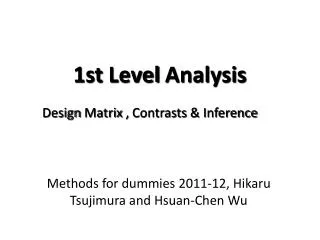
1st level design matrix: 6 sessions per subject
15 auditory contrasts 2 target contrasts 6 movement parameters A regressor, X,= timeseries of expected activation. A = convolved with HRF B = not convolved with HRF Data, Y Y = X + e Betas are calculated for each column of the design matrix 23 betas x 6 sessions = 138 + 6 constants = 144 beta images. A B
The following images are created each time an analysis is performed (1st or 2nd level) • beta images (with associated header), images of estimated regression coefficients (parameter estimate). Combined to produce con. images. • mask.img This defines the search space for the statistical analysis. • ResMS.img An image of the variance of the error (NB: this image is used to produce spmT images). • RPV.img The estimated resels per voxel (not currently used).
1st-level (within-subject) ^ b1 ^ 1 ^ b2 ^ 2 ^ b3 ^ 3 ^ b4 ^ 4 ^ b5 ^ 5 ^ b6 ^ 6 ^ w= within-subject error Beta images contain values related to size of effect. A given voxel in each beta image will have a value related to the size of effect for that explanatory variable. The ‘goodness of fit’ or error term is contained in the ResMS file and is the same for a given voxel within the design matrix regardless of which beta(s) is/are being used to create a con.img. Design efficiency
Mask.img Calculated using the intersection of 3 masks: 1) user specified, 2) Implicit (if a zero in any image then masked for all images) default = yes, 3) Thresholding which can be i) none, ii) absolute, iii) relative to global (80%).
Specify this contrast for each session
Contrast 1: Vowel - baseline
Beta value = % change above global mean. In this design matrix there are 6 repetitions of the condition so these need to be summed. Con. value = summation of all relevant betas.
ResMS.img = residual sum of squares or variance image and is a measure of within-subject error at the 1st level or between-subject error at the 2nd. Con. value is combined with ResMS value at that voxel to produce a T statistic or spm.T.img.
spmT.img Thresholded using the results button.
ci = voxel value in contrast image at voxel i Con= contrast applied to design matrix
ci = voxel value in contrast image at voxel i ConT = contrast applied to design matrix C = Constant term
Efficiency term Contrast specific (See Tom Jenkins’/ Paul Bentley’s slides). ci = voxel value in contrast image at voxel i ConT = contrast applied to design matrix C = Constant term
ci = voxel value in contrast image at voxel i ConT = contrast applied to design matrix C = Constant term
ci = voxel value in contrast image at voxel i ConT = contrast applied to design matrix C = Constant term
Summary • beta images contain information about the size of the effect of interest. • Information about the error variance is held in the ResMS.img. • beta images are linearly combined to produce relevant con. images. • The design matrix, contrast, constant and ResMS.img are subjected to matrix multiplication to produce an estimate of the st.dev. associated with each voxel in the con.img. • The spmT.img are derived from this and are thresholded in the results step.
Contrast 2: Vowel - Tones
Vowel - baseline Tone - baseline Vowel - Tone Vowel – baseline Contrast images for the two classes of stimuli versus baseline and versus each other (linear summation of all relevant betas)
Vowel - baseline Tone - baseline Vowel - Tone spmT images for the two classes of stimuli versus baseline and versus each other (these are not linearly related as the st.dev. of the voxel value in each con.img varies with each contrast).
2nd level analysis – what’s different? • Maths is identical. • Con.img at the first level are output files, at the second level they are both input and output files. • 1st level: variance is within subject, 2nd level: variance is between subject. • Different types of design matrix (3 examples).
Specify 2nd level: One-sample t-test Simplest example, most parsimonious.
Group mask Single subject mask NB: Mask file will only include voxels common to all subjects.
Estimate: Results: Vowel – Tone contrast.
beta.img con.img NB: beta and con images are identical.
spmT.img Plot from voxel shows error variance.
Vowels Formants Tones Specify 2nd level: Full factorial More than one contrast per subject, can cause a problem with sphericity assumptions. Can analyse systematically: simple main effects then interactions. Mask one contrast with another etc.
Specify 2nd level: One-sample t-test Simplest example, most parsimonious
Test with a conjunction term: Which voxels are activated in both contrasts Vowels Formants Tones Plot:
Specify 2nd level: One sample t-test with a covariate added. Test correlations between task specific activations and some other measure (age, performance, etc.). Vectors added here. Needs to be mean corrected by hand. (in this case age squared then mean corrected).
Main effect of grip (1st level analysis event related Correlation between grip and age of subject design: grip vs. rest)
This plot correlates betas related to grip (y-axis) with a measure of age (x-axis)
2nd level analysis summary • Many different ways of entering the contrast images of interest generated by the first level design matrix. • Choice depends primarily on: • Initial study design. • Parsimonious models vs. more complex ones.
volume = defined by mask.img Voxels = volume/8: FDR-corr Resels = calculated from the estimated smoothness (FWHM): FEW-corr
Canonical 152 T1.img STG mask (created in MRIcro. NB: must reorient origin in spm).
SVC summary • p value associated with t and Z scores is dependent on 2 parameters: • Degrees of freedom. • How you choose to correct for multiple comparisons.
Sources • Rik Henson’s slides. • MfD past and present. • SPM manual (D:\spm5\man). • Will Penny.