Download
1 / 57
600 likes | 810 Views
Time-dependent phenomena in quantum transport. E.K.U. Gross. Max-Planck Institute for Microstructure Physics Halle. w eb : http:// users .physik.fu-berlin.de/~ag-gross. c entral region C. left lead L. r ight lead R. Electronic transport: Generic situation.

E N D
Time-dependent phenomena in quantum transport E.K.U. Gross Max-Planck Institute for Microstructure Physics Halle web: http://users.physik.fu-berlin.de/~ag-gross
central region C left lead L right lead R Electronic transport: Generic situation Bias between L and R is turned on: U(t) V for large t A steady current, I, may develop as a result.
central region C left lead L right lead R Electronic transport: Generic situation Bias between L and R is turned on: U(t) V for large t A steady current, I, may develop as a result. Goal 1: Calculate current-voltage characteristics I(V)
central region C left lead L right lead R Electronic transport: Generic situation Bias between L and R is turned on: U(t) V for large t A steady current, I, may develop as a result. Goal 1: Calculate current-voltage characteristics I(V) Goal 2: Analyze how steady state is reached, determine if there is steady state at all and if it is unique
central region C left lead L right lead R Electronic transport: Generic situation Bias between L and R is turned on: U(t) V for large t A steady current, I, may develop as a result. Goal 1: Calculate current-voltage characteristics I(V) Goal 2: Analyze how steady state is reached, determine if there is steady state at all and if it is unique Goal 3: Control path of current through molecule by laser
Control the path of the current with laser right lead left lead
Control the path of the current with laser right lead left lead Necessary: Algorithm to calculate shape of optimal laser pulse with quantum optimal control theory
Outline • Standard Landauer approach (using static DFT ) • Why time-dependent transport? • Computational issues (open, nonperiodic system) • Recovering Landauer steady state within TD framework • Transients and the time-scale of dephasing • Electron pumping • Undamped oscillations associated with bound states • Oscillations associated with Coulomb blockade
central region C left lead L right lead R Standard approach: Landauer formalism plus static DFT Transmission function T(E,V) calculated from static (ground-state) DFT Comparison with experiment: Qualitative agreement, BUT conductance often 1-3 orders of magnitude too high.
Define Green’s functions of the static leads eigenstates of static KS Hamiltonian of the complete system (no periodicity!)
Substitute L and R in equation for central region (HCLGLHLC + HCC + HCRGRHRC) C = E C Effective KS equation for the central region L := HCL GLHLC R := HCR GRHRC g = ( E - HCC - L - R)-1
Chrysazine Relative Total Energies and HOMO-LUMO Gaps Chrysazine (a) Chrysazine (c) 0.0 eV 3.35 eV 1.19 eV 3.77 eV Chrysazine (b) 0.54 eV 3.41 eV
-1.99 -3.39 -4.10 -4.49 -6.28 -6.47 -6.75 -7.21 -7.38 -7.36 -7.59 Energy (eV)
Possible use: Optical switch A.G. Zacarias, E.K.U.G., Theor. Chem. Accounts 125, 535 (2010)
Summary of standard approach • Use ground-state DFT within Landauer formalism • Fix left and right chemical potentials • Solve self-consistently for KS Green’s function • Transmission function has resonances at KS levels • No empirical parameters, suggests confidence level of ground-state DFT calculations
Two conceptual issues: Assumption that upon switching-on the bias a steady state evolves
Two conceptual issues: Assumption that upon switching-on the bias a steady state evolves Steady state is treated with ground-state DFT In particular, transmission function has peaks at the excitation energies of the gs KS potential.
Two conceptual issues: Assumption that upon switching-on the bias a steady state evolves Steady state is treated with ground-state DFT In particular, transmission function has peaks at the excitation energies of the gs KS potential. Hence, resonant tunneling occurs at wrong energies (even with the exact xc functional of gs DFT).
Two conceptual issues: • Assumption that upon switching-on the bias • a steady state evolves • Steady state is treated with ground-state DFT • In particular, transmission function has peaks • at the excitation energies of the gs KS potential. • Hence, resonant tunneling occurs at wrong energies • (even with the exact xc functional of gs DFT). • One practical aspect: • TD external fields, AC bias, laser control, etc, cannot be treated within the static approach
Three different ab-initio approaches • TD many-body perturbation theory (Kadanoff-Baym equation) • TD denstity-functional theory (TD Kohn-Sham equation) • TD wave-function approaches (TD many-body Schrödinger equation)
Three different ab-initio approaches • TD many-body perturbation theory (Kadanoff-Baym equation) • --theory straightforward • --numerically difficult • TD denstity-functional theory (TD Kohn-Sham equation) • TD wave-function approaches (TD many-body Schrödinger equation)
Three different ab-initio approaches • TD many-body perturbation theory (Kadanoff-Baym equation) • --theory straightforward • --numerically difficult • TD denstity-functional theory (TD Kohn-Sham equation) • --theory complicated (xc functional) • --numerically simple • TD wave-function approaches (TD many-body Schrödinger equation)
Three different ab-initio approaches • TD many-body perturbation theory (Kadanoff-Baym equation) • --theory straightforward • --numerically difficult • TD denstity-functional theory (TD Kohn-Sham equation) • --theory complicated (xc functional) • --numerically simple • TD wave-function approaches (TD many-body Schrödinger equation) • --theory known • --numerically very difficult • --most accurate of all (when feasible)
Three different ab-initio approaches • TD many-body perturbation theory (Kadanoff-Baym equation) • --theory straightforward • --numerically difficult • TD denstity-functional theory (TD Kohn-Sham equation) • --theory complicated (xc functional) • --numerically simple • TD wave-function approaches (TD many-body Schrödinger equation) • --theory known • --numerically very difficult • --most accurate of all (when feasible)
Electronic transport with TDDFT central region C left lead L right lead R vxc[ (r’t’)](r t) TDKS equation (E. Runge, EKUG, PRL 52, 997 (1984))
Electronic transport with TDDFT central region C left lead L right lead R TDKS equation
is purely kinetic, because KS potential is local are time-independent Propagate TDKS equation on spatial grid with grid points r1, r2, … in region A (A = L, C, R)
L L C R R Next step: Solve inhomogeneous Schrödinger equations , for L, R using Green’s functions of L, R, leads Hence:
r.h.s. of solution of hom. SE r.h.s. of solution of hom. SE L R C insert this in equation Define Green’s Functions of left and right leads: explicity:
Effective TDKS Equation for the central (molecular) region S. Kurth, G. Stefanucci, C.O. Almbladh, A. Rubio, E.K.U.G., Phys. Rev. B 72, 035308 (2005) source term: L → C and R → C charge injection memory term: C → L → C and C → R → C hopping Note: So far, no approximation has been made.
Necessary input to start time propagation: • lead Green’s functions GL, GR • initial orbitals C(0) in central region as initial condition for time propagation
Calculation of lead Green’s functions: Simplest situation: Bias acts as spatially uniform potential in leads (instantaneous metallic screening) likewise total potential drop across central region
initial orbitals in C region eigenstates of static KS Hamiltonian of the complete system Gives effective static KS equation for central region In the traditional Landauer + static DFT approach, this equation is used to calculate the transmission function. Here we use it only to calculate the initial states in the C-region.
Numerical examples for non-interacting electrons Recovering the Landauer steady state left lead central region right lead U V(x) U Time evolution of current in response to bias switched on at time t = 0, Fermi energy F = 0.3 a.u. Steady state coincides with Landauer formula and is reached after a few femtoseconds
Transients Solid lines: Broken lines: Sudden switching central region left lead right lead V(x) U0 barrier height: 0.5 a.u. F= 0.3 a.u. same steady state!
ELECTRON PUMP Device which generates a net current between two electrodes (with no static bias) by applying a time-dependent potential in the device region Recent experimental realization : Pumping through carbon nanotube by surface acoustic waves on piezoelectric surface (Leek et al, PRL 95, 256802 (2005))
Pumping through a square barrier (of height 0.5 a.u.) using a travelling wave in device region U(x,t) = Uosin(kx-ωt) (k = 1.6 a.u., ω = 0.2 a.u. Fermi energy = 0.3 a.u.) Archimedes’ screw: patent 200 b.c.
Experimental result: Current flows in direction opposite to sound wave
Bound state oscillations and memory effects Analytical: G. Stefanucci, Phys. Rev. B, 195115 (2007)) Numerical: E. Khosravi, S. Kurth, G. Stefanucci, E.K.U.G., Appl. Phys. A93, 355 (2008), and Phys. Chem. Chem. Phys. 11, 4535 (2009) If Hamiltonian of a (non-interacting) biased system in the long-time limit supports two or more bound states then current has steady, I(S), and dynamical, I(D), parts: Sum over bound states of biased Hamiltonian Note: - bb’ depends on history of TD Hamiltonian (memory!) Questions: -- How large is I(D) vs I(S)? -- How pronounced is history dependence?
History dependence of undamped oscillations 1-D model: start with flat potential, switch on constant bias, wait until transients die out, switch on gate potential with different switching times to create two bound states note: amplitude of bound-state oscillations may not be small compared to steady-state current
amplitude of current oscillations as function of switching time of gate question: what is the physical reason behind the maximum of oscillation amplitude ?
So far: systems without e-e interaction Next step: TDKS, i.e. inclusion of e-e- interaction via approximate xc potential time-dependent picture of Coulomb blockade
Solve TDKS equations (instead of fully interacting problem): LDA functional for vxc is available from exact Bethe-ansatz solution of the 1D Hubbard model. N.A. Lima, M.F. Silva, L.N. Oliveira, K. Capelle, PRL 90, 146402 (2003)
We use this functional as Adiabatic LDA (ALDA) in the TD simulations. Note: has a discontinuity at n = 1
S. Kurth, G. Stefanucci, E. Khosravi, C. Verdozzi, E.K.U.G., Phys. Rev. Lett. 104, 236801 (2010)
Is this Coulomb blockade? Steady-state equation has no solution in this parameter regime (if vKS has sharp discontinuity)!