Download
1 / 63
630 likes | 758 Views
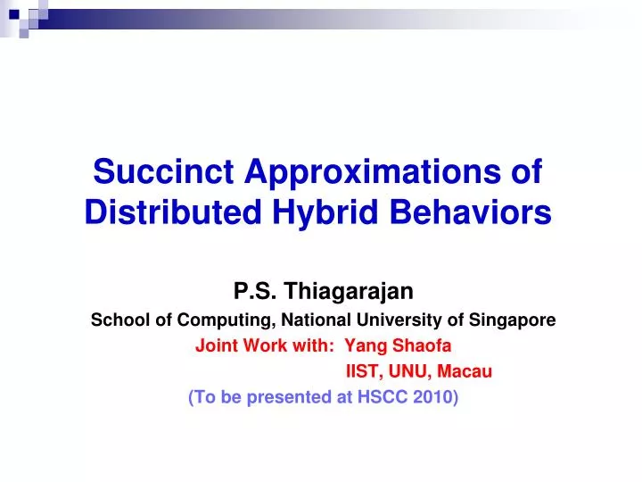
Succinct Approximations of Distributed Hybrid Behaviors. P.S. Thiagarajan School of Computing, National University of Singapore Joint Work with: Yang Shaofa IIST, UNU, Macau (To be presented at HSCC 2010). Hybrid Automata. Hybrid behaviors:

E N D
Succinct Approximations of Distributed Hybrid Behaviors P.S. Thiagarajan School of Computing, National University of Singapore Joint Work with: Yang Shaofa IIST, UNU, Macau (To be presented at HSCC 2010)
Hybrid Automata • Hybrid behaviors: • Mode-specific continuous dynamics + discrete mode changes • Standard model: Hybrid Automata • Piecewise constant rates • Rectangular guards
Piecewise Constant Rates A A {x1, x2, x3} g B B D D B (x1, x2, x3) = (2, -3.5, 1) dx1/dt = 2 x1(t) = 2t + x1(0) dx2/dt = -3.5 dx3/dt = 1 C C
Rectangular Guards A g B D C x2 x c | x c | ’ x1
Initial Regions (x1 2 x1 1) (x2 3.5 x2 0.5) A x2 g x1 B D C
Highly Expressive • Piecewise constant rates; rectangular guards • The control state (mode) reachability problem is undecidable. • Given qf, Whether there exists a trajectory (q0, x0) (q1, x1) ……. (qm, xm) such that qm = qf • q0 = initial mode; x0in initial region. • HKPV’95
(q4, x4) (q1, x1) g (q0) (q2, x2) (q0, x0) (q3, x3)
Two main ways to circumvent undecidability • If its rate changes as the result of a mode change, • Reset the value of a variable to a pre-determined region
Hybrid Automata with resets. VF x 5 dx/dt = 3 dx/dt = -1.5 5 x 2.8 2.8 VD
Hybrid Automata with resets. VF x 5 x [2, 4] dx/dt = 3 dx/dt = -1.5 5 x 2.8 2.8 VD
Control Applications PLANT actuators Sensors Digital Controller The reset assumption is untenable.
PLANT actuators Sensors Digital Controller [HK’97]: Discrete time assumption. The plant state is observed only at (periodic) discrete time points T0 T1 T2 ….. T i+1 – Ti =
Discrete time behaviors • The discrete time behavior of a hybrid automaton: • Q : The set of modes • q0 q1 …qm is a state sequenceiff there exists a run (q0, v0, ) (q1, v1) … (qm, vm) of the automaton. • The discrete time behavior of Aut is • L(Aut) Q* • the set of state sequences of Aut.
[HK’97]: • The discrete time behavior of (piecewise constant + rectangular guards) an hybrid automaton is regular. • A finite state automaton representing this language can be effectively constructed. • Discrete time behavior is an approximation. With fast enough sampling, it is a good approximation.
[AT’04]: The discrete time behavior of an hybrid automaton is regular even with delays in sensing and actuating (laziness)
g k k-1 g g + g The value of xi reported at t = k is the value at some t’ in [(k-1)+ g, (k-1)+g +g] g and g are fixed rationals
h h + h k k+1 h If a mode change takes place at t = k is then xi starts evolving at ’(xi) at some t’ in [k+ h, k+h + h] h and h are fixed rationals.
Global Hybrid Automata PLANT Sensors Actuators Digital Controller (x1) ? x1 (x2) ? x2 (x3) ? x3
Distributed Hybrid Automata PLANT Sensors Actuators ? x1 p1 (x1) ? x2 p2 (x2) p3 (x3) ? x3
No explicit communication between the automata.. However, coordination through the shared memory of the plant’s state space.
The Communictaion graph of DHA Obs(p) --- The set of variables observed by p Ctl(p) --- The set of variables controlled by p Ctl(p) Ctl(q) = Nbr(p) = Obs(p) Ctl(p)
[(s01), (s02), (s03)] [(s01, v01), (s02, v02), (s03, v03)]
[(s21, v21), (s22, v22), (s23, v23)] [(s11, v11), (s12, v12), (s13, v13)] [(s01), (s02), (s03)] [(s01, v01), (s02, v02), (s03, v03)]
[(s21, v21), (s22, v22), (s23, v23)] [(s11, v11), (s12, v12), (s13, v13)] [(s01), (s02), (s03)] [(s31, v31), (s32, v32), (s33, v33)] [(s01, v01), (s02, v02), (s03, v03)]
[(s21, v21), (s22, v22), (s23, v23)] [(s41, v41), (s42, v42), (s43, v43)] [(s11, v11), (s12, v12), (s13, v13)] [(s01), (s02), (s03)] [(s31, v31), (s32, v32), (s33, v33)] [(s01, v01), (s02, v02), (s03, v03)]
Discrete time behavior: (Global) state sequences [s01, s02, s03] [s11,s12,s13] [s21, s22, s23] [s31, s32, s33] . . . .
Discrete time behaviors • The discrete time behavior of DHA is • L(DHA) (Sp1 Sp2 ….. Spn)* • the set of global state sequences of DHA. • L(DHA) is regular?
Discrete time behaviors • The discrete time behavior of DHA is • L(DHA) (Sp1 Sp2 ….. Spn)* • the set of global state sequences of DHA. • L(DHA) is regular? • Yes. Construct the (syntactic product) AUT of DHA. • AUT will have piecewise constant rates and rectangular guards. Hence…..
Global HA Network of HAs Syntactic product Discretization m ---- the number of component automata in DHA The size of DHA will be linear in m The size of AUT will be exponential in m. Can we do better? Global FSA
Network of HAs Global HA Syntactic Product Local discretization Discretization Product Global FSA Network of FSAs
Network of HAs Local discretization Global FSA Network of FSAs
Location node Variable node For each node, construct an FSA Each FSA will “read” from all its neighbor FSAs to make its moves. Nbr(p) = Ctl(p) Obs(p) Nbr(x) = {p | x Ctl(p) Obs(p) }
Autx • Autxwill keep track of the current value of x • CTL(x) = p if x Ctl(p) • A move of Autx: • read the current rate of x from AutCTL(x) and update the current value of x • Can only keep bounded information • Quotient the value space of x
Quotienting the value space of x vmax vmin
Quotienting the value space of x c c’ c, c’ , ., . ., the constants that appear in some guard
Quotienting the value space of x , ’ ….. rates of x associated with modes in AUTCTL(x) || |’| Find the largest positive rational that evenly divides all these rationals . Use it to divide [vmin, vmax] into uniform intervals
Quotionting the value space of x ( ) ( ) A move of Autx: If Autx is in state I and CTL(x) = p and Autp’s state is then Autx moves from I to I’ = (I)
( ) ( ) ( ) I’ I (s2, 2) (s1, 1) I Aut(x1) I’ I’ = 1(I)
I1 I2 (s2, 2) I3 (s2, 2) Aut (p2 ) (v1, v3) satisfies g for some (v1, v3) in I1 I3 g (s’2, ’2) (s’2, ’2)
Aut(x1) Aut(p3) Aut(p1) Aut(x3) Aut(x2) Aut(p2) Each automaton will have a parity bit. This bit flips every time the automaton makes a move. Initially all the parities are 0. A variable node automaton makes a move only when its parity is the same as all its neighbors’ A location node automaton makes a move only when its parity is different from all its neighbors.
Aut(x1) Aut(p3) Aut(p1) Aut(x3) Aut(x2) Aut(p2)
Aut(x1) Aut(p3) Aut(p1) Aut(x3) Aut(x2) Aut(p2)
Aut(x1) Aut(p3) Aut(p1) Aut(x3) Aut(x2) Aut(p2)
Aut(x1) Aut(p3) Aut(p1) Aut(x3) Aut(x2) Aut(p2)
Aut(x1) Aut(p3) Aut(p1) Aut(x3) Aut(x2) Aut(p2)
Aut(x1) Aut(p3) Aut(p1) Aut(x3) Aut(x2) Aut(p2)
Aut(x1) Aut(p3) Aut(p1) Aut(x3) Aut(x2) Aut(p2)
Aut(x1) Aut(p3) Aut(p1) Aut(x3) Aut(x2) Aut(p2)